Hello! My name is Donghao Hong, a Master’s student in Electrical and Computer Engineering (ECE).
My academic interests include robotics, embedded systems, and autonomous systems.
This website documents my coursework, labs, and projects for ECE 5160 Fast Robots.
The goal is to program the Artemis board and establish reliable bidirectional
Bluetooth Low Energy (BLE) communication between the board and a laptop
for command execution and data exchange.
Lab 1A
Prelab
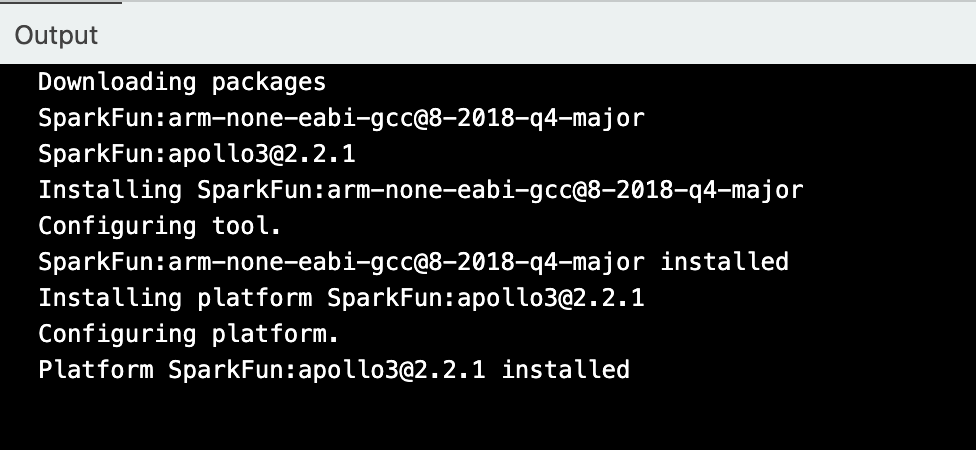
I set up the Arduino IDE and installed the SparkFun Apollo3 board support package.
Task 1: Setup
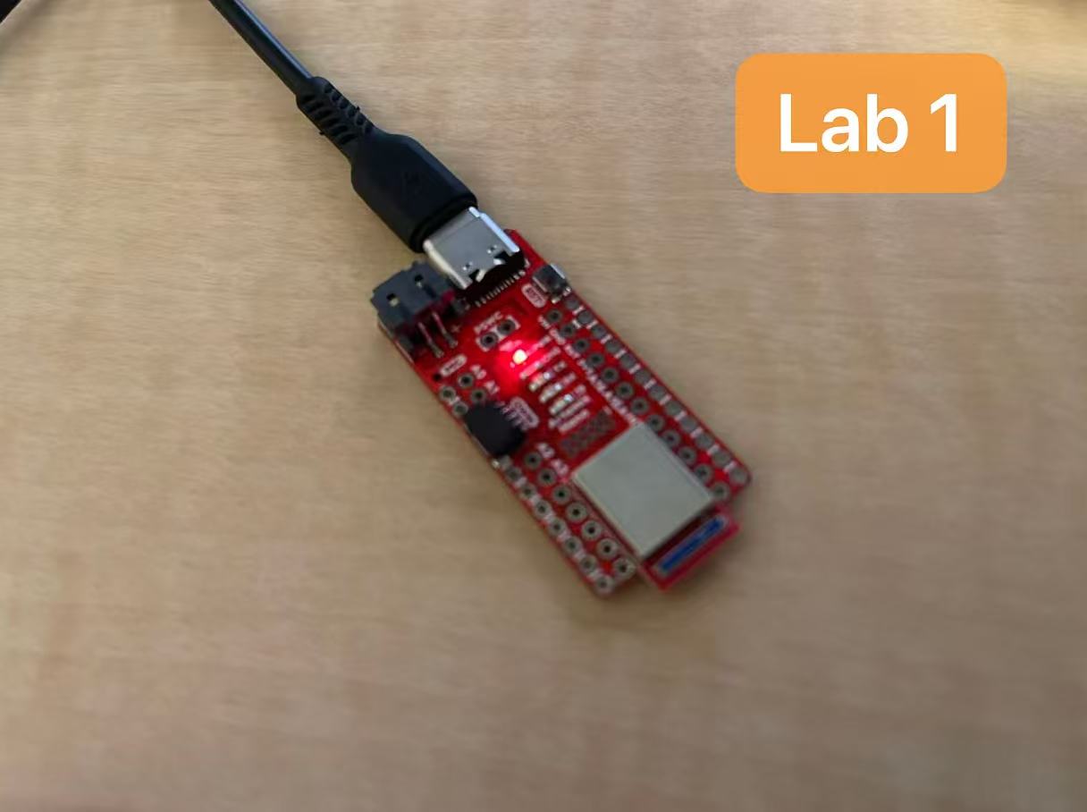
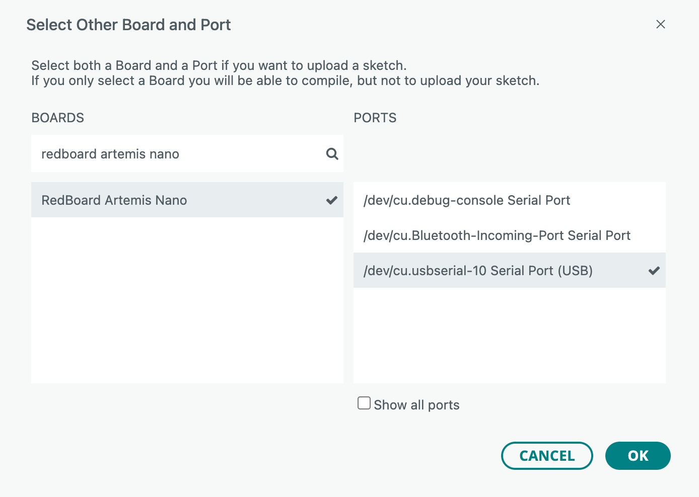
I connected the Artemis board to the computer and selected the RedBoard Artemis Nano
and the correct USB serial port in the Arduino IDE.
Task 2: Blink
The onboard LED repeatedly turned on and off at a fixed interval, producing a steady blinking pattern.
Task 3: Serial
Text input from the computer was received by the Artemis board and printed in the Serial Monitor, confirming successful serial communication.
Task 4: AnalogRead
When the Artemis board was held by hand, the reported temperature values gradually increased as heat was transferred from the hand to the board. Specifically, the temperature reading rose from approximately 33956 to 34182 over time, demonstrating that the onboard temperature sensor responded to changes in environmental temperature.
Task 5: PDM
When whistling near the Artemis board, the detected frequency exhibited a sudden increase in magnitude. Once the whistling stopped, the frequency values returned to their baseline levels, indicating that the onboard PDM microphone correctly responded to changes in sound input.
Additional Task (5000-level)
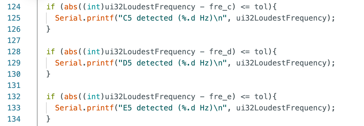
For the 5000-level additional task, I extended the PDM + FFT example to detect specific tones by
finding the dominant frequency peak and comparing it against three target notes (C5, D5, and E5)
within a small tolerance. To generate known test tones, I downloaded an app called Tuner T1,
which can play pure tones at user-specified frequencies. When playing the corresponding frequencies,
the Artemis code correctly reported C5, D5, and E5 over serial,
confirming that the frequency detection logic worked as intended.
Lab 1B
Prelab
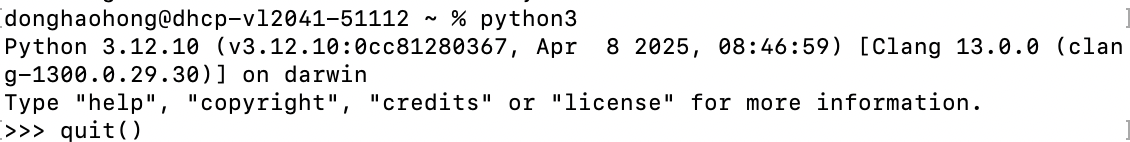
Before starting the lab, I verified that Python was correctly installed on my system by launching the Python interpreter from the terminal. This confirmed that a suitable Python environment was available for running the host-side BLE scripts required for the experiment.
I then activated the provided Fast Robots BLE virtual environment, which contains the necessary dependencies for Bluetooth communication with the Artemis board.
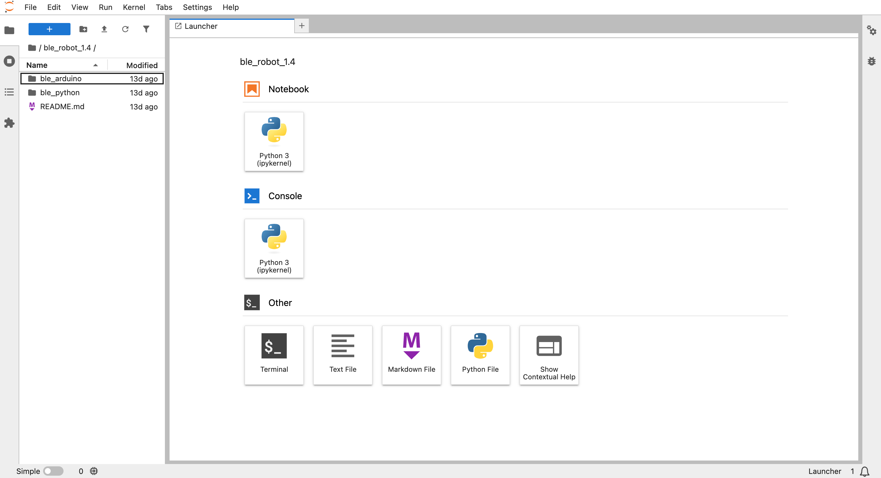
Finally, I launched Jupyter Notebook and confirmed that the BLE project directory and Python kernel were correctly loaded.
Configurations
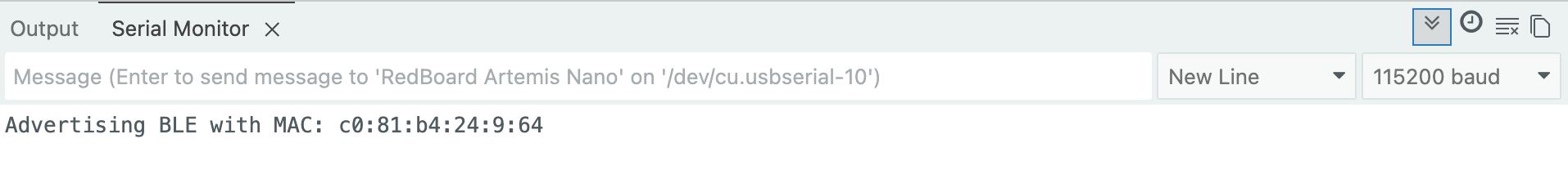
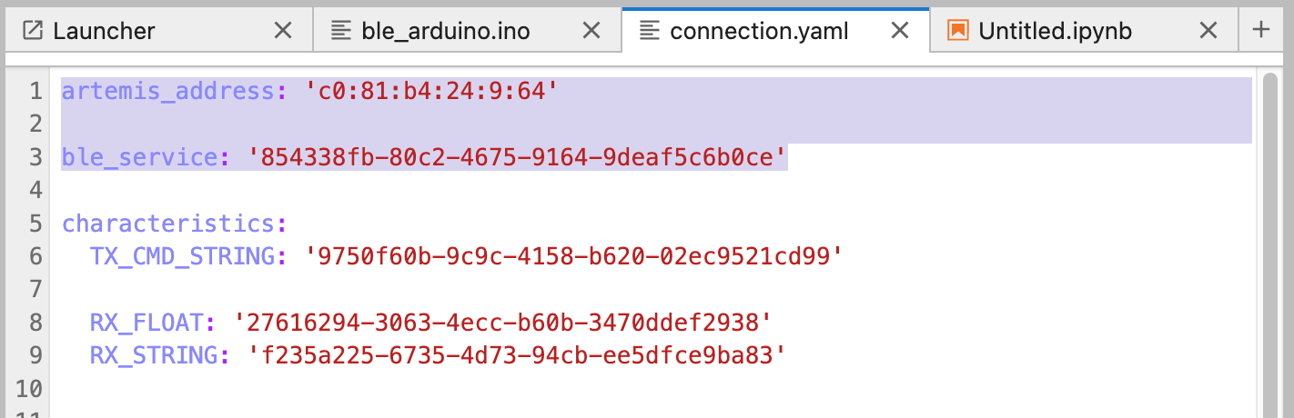
After uploading the ble_arduino.ino sketch to the Artemis Nano board, the device began advertising over BLE and printed its MAC address to the serial monitor. This MAC address was then copied into the connection.yaml file by replacing the artemis_address field, allowing the host computer to identify and connect to the correct Artemis device.
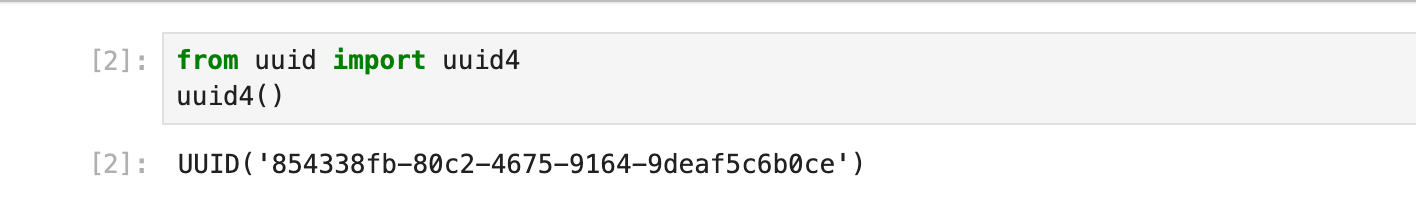
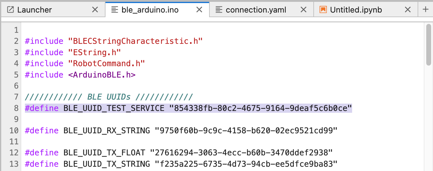
I generated a unique BLE service UUID using a Python command. This UUID was used to define a custom
BLE service for communication between the Artemis board and the host computer.
The generated UUID was then inserted into both the ble_arduino.ino firmware and the
connection.yaml configuration file on the host side. Ensuring that the BLE service and
characteristic UUIDs matched on both sides allowed the Python scripts to successfully discover
and communicate with the Artemis board.
Task 1: ECHO
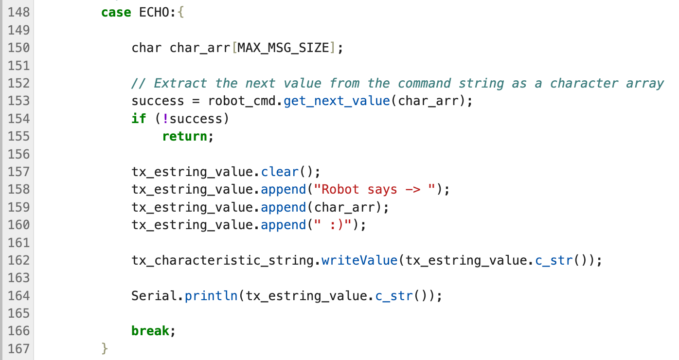
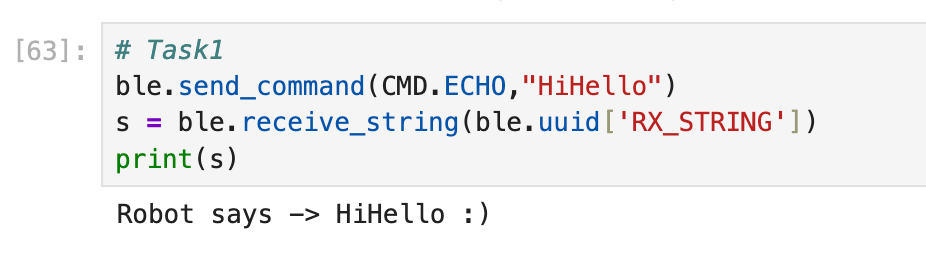
On the Artemis side, the ECHO command extracts the incoming string and sends it backover BLE by writing a formatted response to the string characteristic.
From Jupyter, I sent an ECHO command and successfully received the same string in theresponse, confirming reliable bidirectional BLE communication.
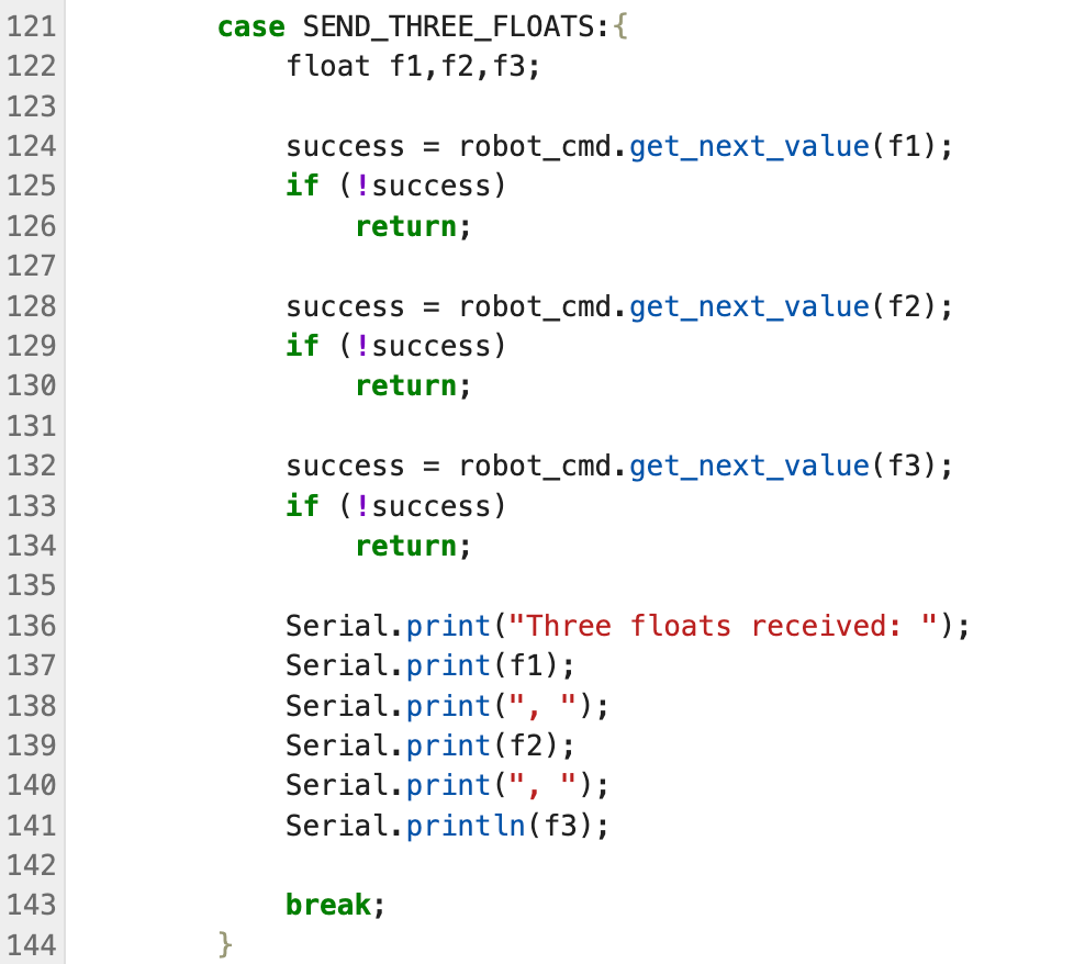
Task 2: SEND_THREE_FLOATS
For this task, I implemented a SEND_THREE_FLOATS command to transmit three floating-point values from the host
computer to the Artemis board over BLE. On the Arduino side, the command handler sequentially parses three float values
from the incoming command string using robot_cmd.get_next_value() and prints them to the serial monitor for verification.
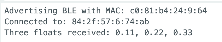
From Jupyter, I sent the command with three floats encoded as a single string, and the Artemis board correctly received
and decoded all three values, confirming reliable multi-parameter data transmission over BLE.
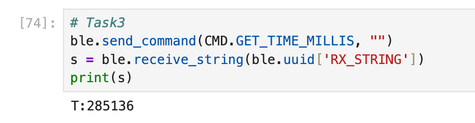
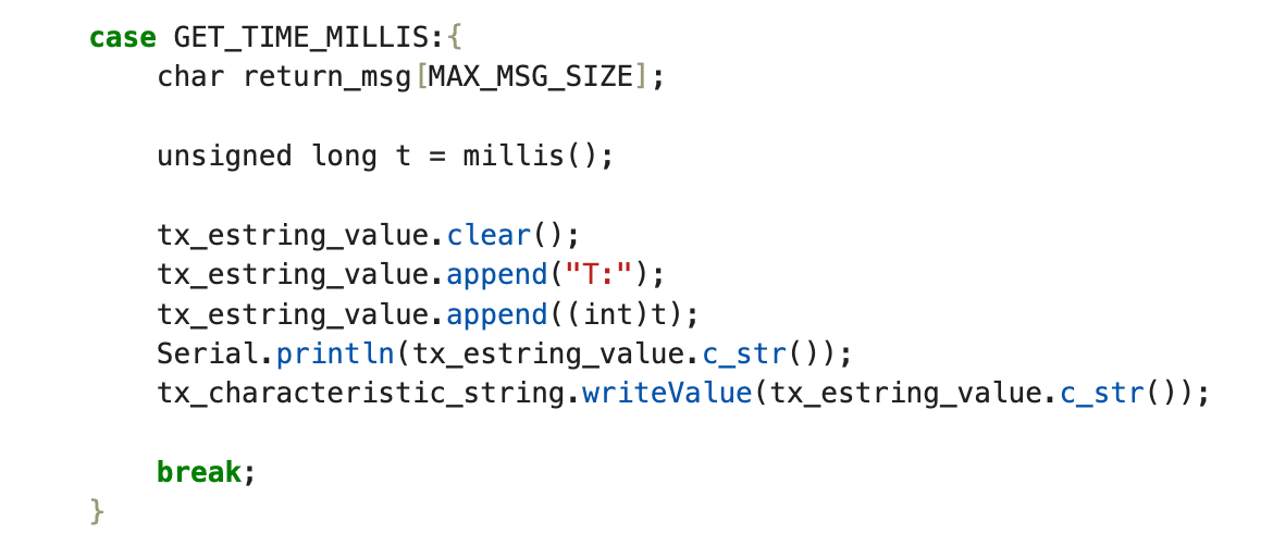
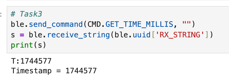
Task 3: GET_TIME_MILLIS
On the Arduino side, a GET_TIME_MILLIS command was implemented to return the current value of
millis(), representing the elapsed time since startup. The value was packaged as a string and
sent back over BLE. From Jupyter, the command was issued and the returned timestamp
(e.g., T:285136) was successfully received, verifying correct BLE communication.
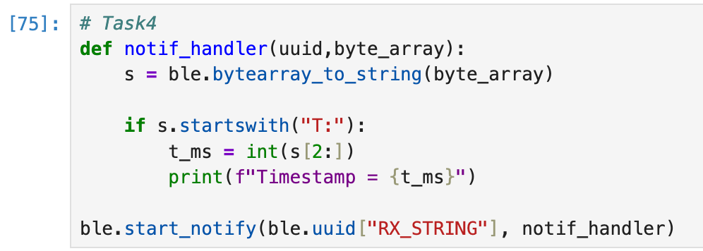
Task 4: Notification Handler
On the Python side, a notification handler was registered for the RX_STRING characteristic.
The handler converts incoming byte arrays into strings and parses messages starting with
"T:" as timestamps. Once notifications were enabled, the Artemis board was able
to asynchronously send time data, which was immediately received and printed in Jupyter
without explicitly polling for responses.
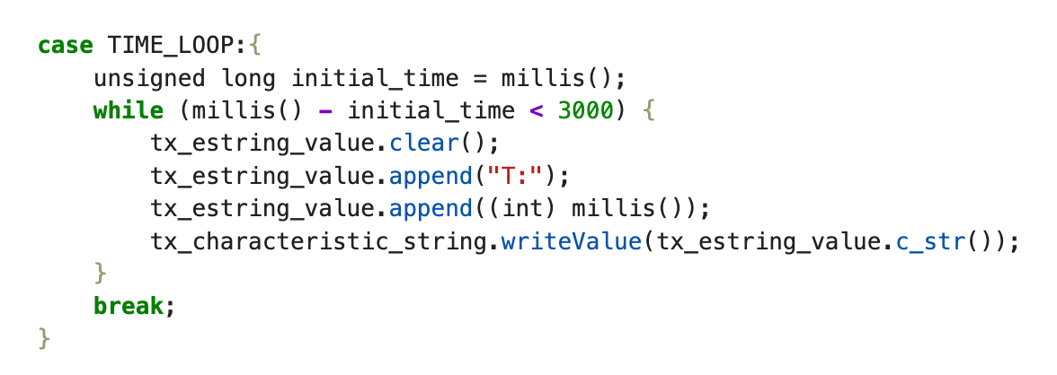
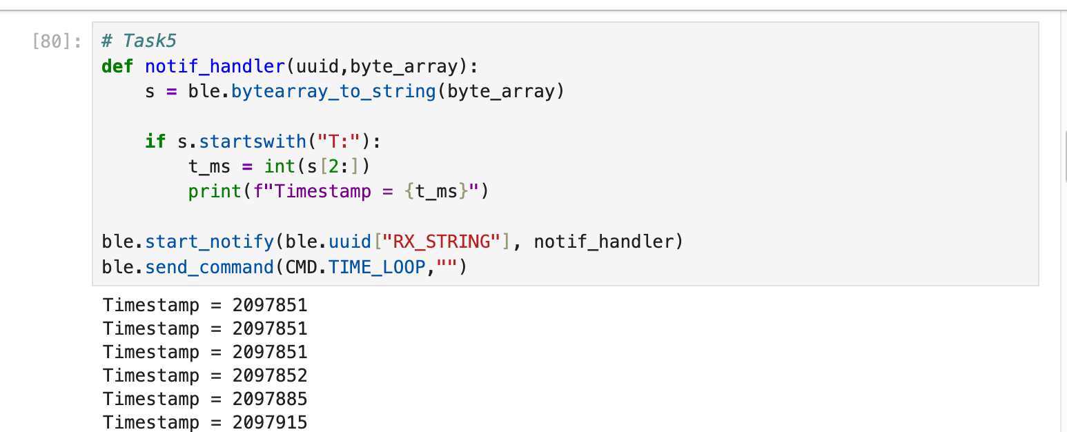
Task 5: Time Loop
In this method, the Artemis continuously reads the current timestamp (ms) inside a while loop and
immediately transmits it to the laptop over BLE on every iteration.
On the host side, I used a notification callback to receive and parse the incoming T:<millis> messages in real time.
Pros (real-time streaming):
Low latency — timestamps arrive at the laptop almost immediately.
Simple and intuitive implementation, convenient for debugging and live inspection.
No need to buffer a large dataset on the microcontroller (low RAM usage).
Cons (real-time streaming):
Throughput is limited by BLE bandwidth and host-side processing.
At higher rates, repeated timestamps and/or dropped messages can occur.
BLE sending + string formatting adds overhead and slows down the sampling loop.
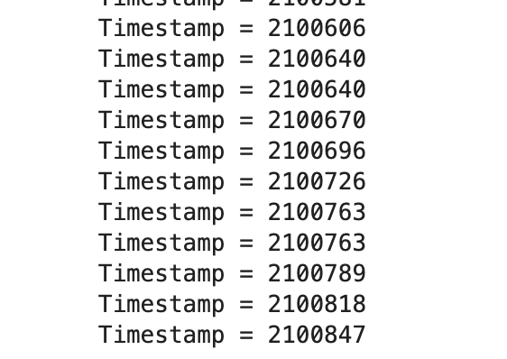
In my test, the board streamed data for about 3 s and I received 214 timestamps.
Each message was about 10 bytes, so the effective rate was
214 / 3 ≈ 71 msg/s, i.e., approximately 71 × 10 ≈ 710 bytes/s.
(The timestamp output was long, so I only included the beginning and the end of the stream.)
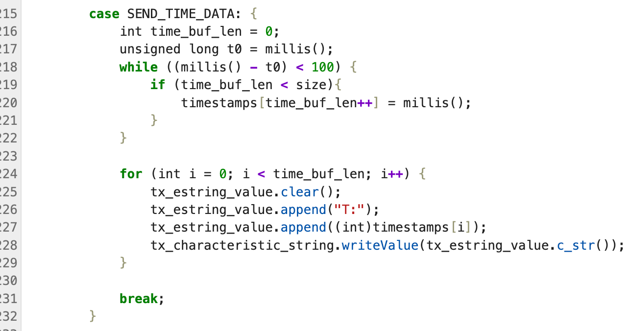
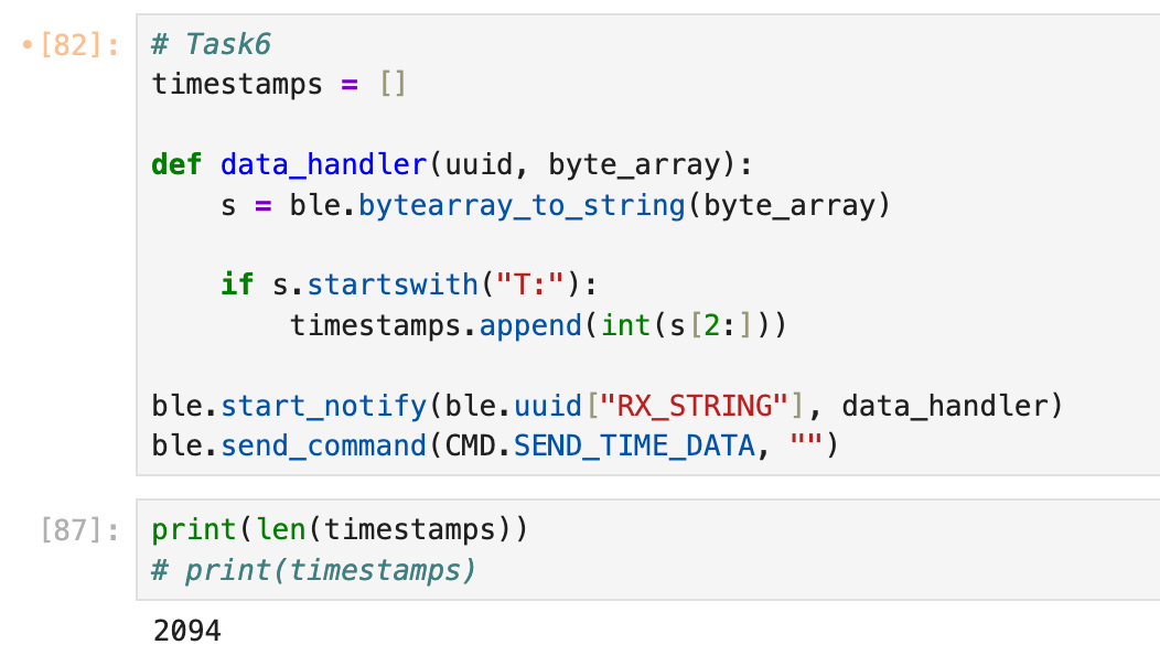
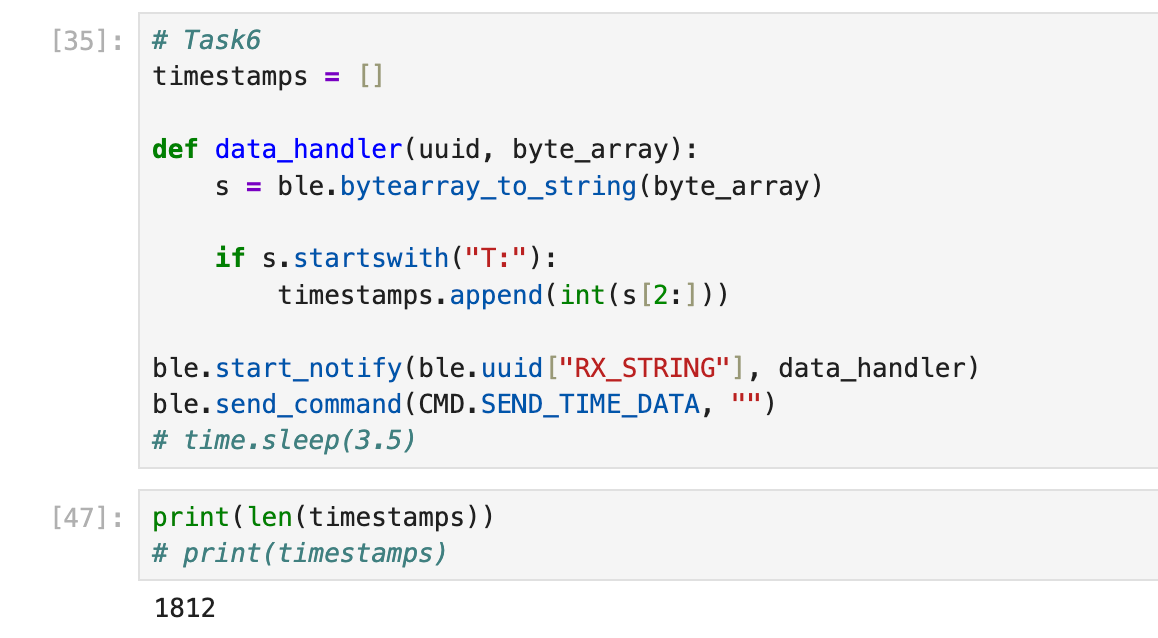
Task 6: Time Array
In this task, the Artemis board first collected timestamps into a local array for a fixed duration
(100 ms) and then transmitted the buffered data to the computer over BLE. On the host side, a
notification handler parsed each T:<millis> message and appended the values to a Python list;
in this run, a total of 2094 timestamps were received.
To prevent buffer overflow on the microcontroller, I added a simple guard:
before writing into the timestamp array, the code checks
if (time_buf_len < size). If the buffer reaches its maximum capacity, no additional samples are
stored, ensuring the firmware never writes past the allocated array bounds.
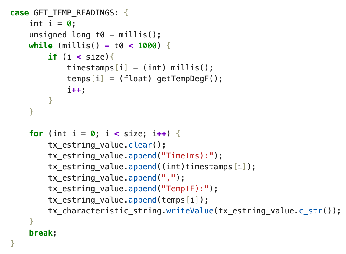
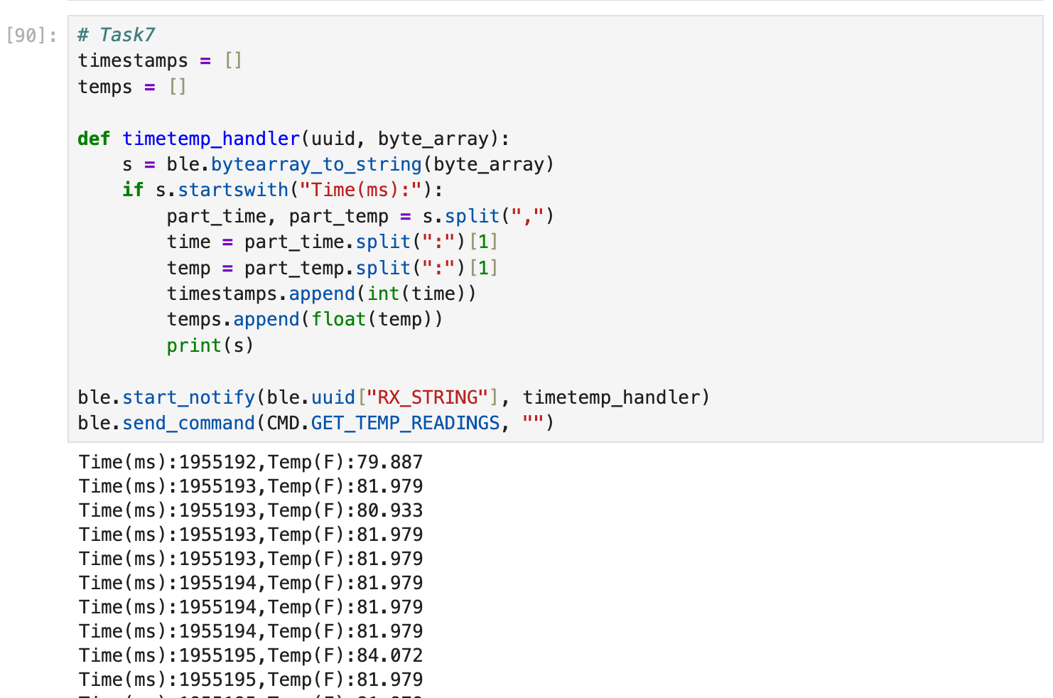
Task 7: Temperature Array
For this task, the Artemis collected paired timestamp and temperature readings in arrays for a fixed duration,
then sent the buffered data to the laptop over BLE. On the Python side, a notification handler parsed each message in the format
Time(ms):...,Temp(F):... and appended the values into timestamps and temps lists for later analysis.
This approach separates data acquisition from transmission, allowing the microcontroller to sample the sensor continuously
while the host computer focuses on parsing and processing the received data.
Task 8: Comparison between the Two Methods
Method 1 (Task 5): real-time streaming. In this approach, the Artemis continuously reads the current timestamp (ms) inside a
while loop and immediately transmits each sample to the laptop over BLE. On the host side, a notification callback receives and
processes the data in real time.
Pros: low latency and near real-time visibility; straightforward implementation that is convenient for debugging and monitoring;
minimal RAM usage since data is not buffered on the microcontroller.
Cons: throughput is limited by BLE and host-side processing; at high sampling rates, repeated timestamps or dropped messages can occur;
BLE transmission and string formatting overhead slows down the loop execution.
Method 2 (Task 6/7): local buffering then batch transfer. In this approach, the Artemis does not communicate over BLE during sampling.
Instead, it stores timestamps (and sensor data) in local arrays, and only after the sampling window ends does it send the buffered data to the laptop
for parsing and analysis.
Pros: faster sampling because the loop avoids BLE overhead; better suited for short bursts of high-frequency data collection; improved
reliability because samples are stored locally before transmission.
Cons: no real-time visibility during sampling (added latency); buffer size is constrained by available RAM; requires extra logic to manage
the buffer and the send-back process.
When to use which: If you need real-time monitoring, debugging, or online control, Method 1 is preferable due to its low latency and
simplicity. If you need high-rate sampling for offline analysis or want to maximize data completeness, Method 2 is preferable because sampling is almost
unaffected by BLE communication overhead (although the upload phase is still limited by BLE throughput).
Sampling speed (Method 2): Over a 0.1 s sampling window, the board recorded 1812 timestamps, which corresponds to
1812 / 0.1 = 18120 samples/s. If we approximate each sample message as ~10 bytes, the implied data rate is
18120 × 10 ≈ 181200 bytes/s.
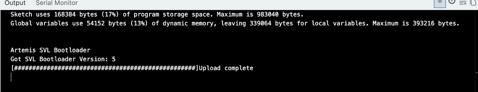
How much can be buffered without exhausting RAM? The Artemis board has 384 kB RAM:
384 × 1024 = 393,216 bytes. The compiled output shows global variables use 54,152 bytes, leaving
339,064 bytes available.
Case A (Task 6, timestamps only): one unsigned long timestamp is 4 bytes, so approximately
339,064 / 4 ≈ 84,766 timestamps.
Case B (Task 7, timestamp + temperature): timestamp 4 bytes + temperature float 4 bytes = 8 bytes per record, so approximately
339,064 / 8 ≈ 42,383 records.
Additional Task (5000 - Level Students)
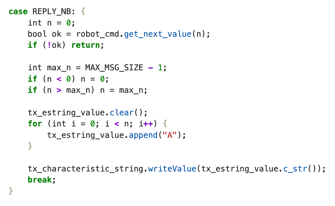
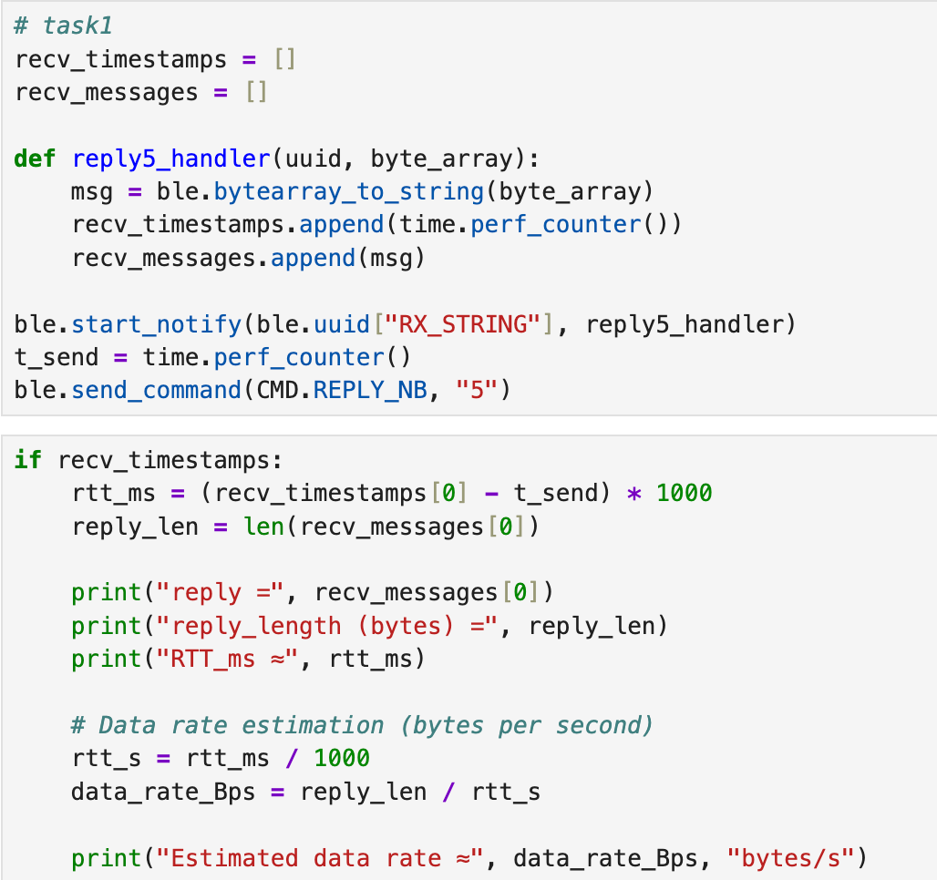
Task 1: Effective Data Rate And Overhead
In this experiment, the laptop sent a request to the Artemis using REPLY_NB, and the Artemis replied with a string
containing n characters. On the Python side, I recorded the send timestamp (t_send) and the first receive
timestamp from the notification callback, then estimated the round-trip time (RTT). Using the reply payload length (bytes) divided by
RTT (seconds), I computed an approximate effective data rate in bytes/s.
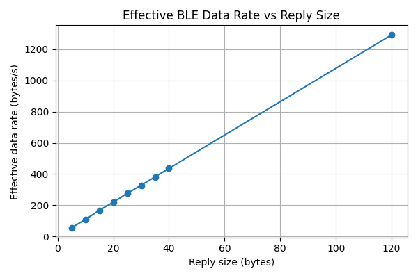
The results show that many small packets introduce significant overhead: RTT stays roughly constant (~90–93 ms) while payload size increases,
so the effective throughput rises as the reply becomes larger. This suggests that using a larger reply amortizes the fixed BLE/processing overhead
and improves effective data rate.
Reply length (bytes)
RTT (ms)
Estimated data rate (bytes/s)
5
91.429
54.687
10
91.838
108.888
15
89.566
167.474
20
91.469
218.652
25
90.652
275.781
30
91.467
327.986
35
91.816
381.196
40
91.779
435.828
120
92.842
1292.520
The plot above summarizes the trend: with a roughly constant RTT, larger replies achieve higher effective throughput. Therefore,
if the application can tolerate buffering (or sending fewer, larger packets), it can significantly reduce the per-message overhead
and improve overall BLE efficiency.
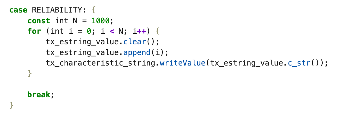
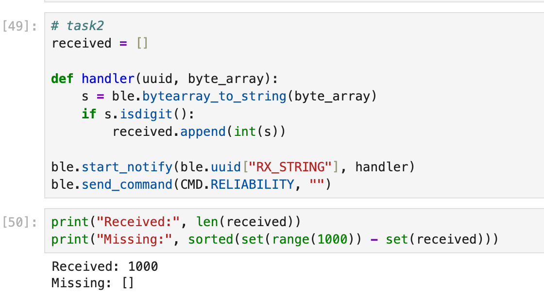
Task 2: Reliability
In this task, the Artemis board was commanded to transmit a sequence of
1000 monotonically increasing integers over BLE as quickly as possible.
On the microcontroller side, the values were sent in a tight loop using BLE
notifications. On the host computer, a Python notification handler parsed each
incoming message and stored the received integers in a list.
After the transmission completed, the received values were compared against
the expected range [0, 999]. As shown in the results, the computer successfully
received all 1000 messages, and the set difference check confirmed that
no data was missing.
This experiment indicates that at the tested transmission rate, the BLE link
between the Artemis board and the host computer was reliable, and the host was
able to process all incoming notifications without packet loss.
Discussion
In this lab, I learned how to configure BLE services and characteristics on the Artemis
board and how to exchange data reliably with a host computer using commands and notifications.
I also observed how BLE communication overhead directly impacts achievable sampling rates.
Lab 2: IMU
The purpose of this lab is to add the IMU to your robot, start running the Artemis+sensors from a battery, and record a stunt on your RC robot.
Setup the IMU
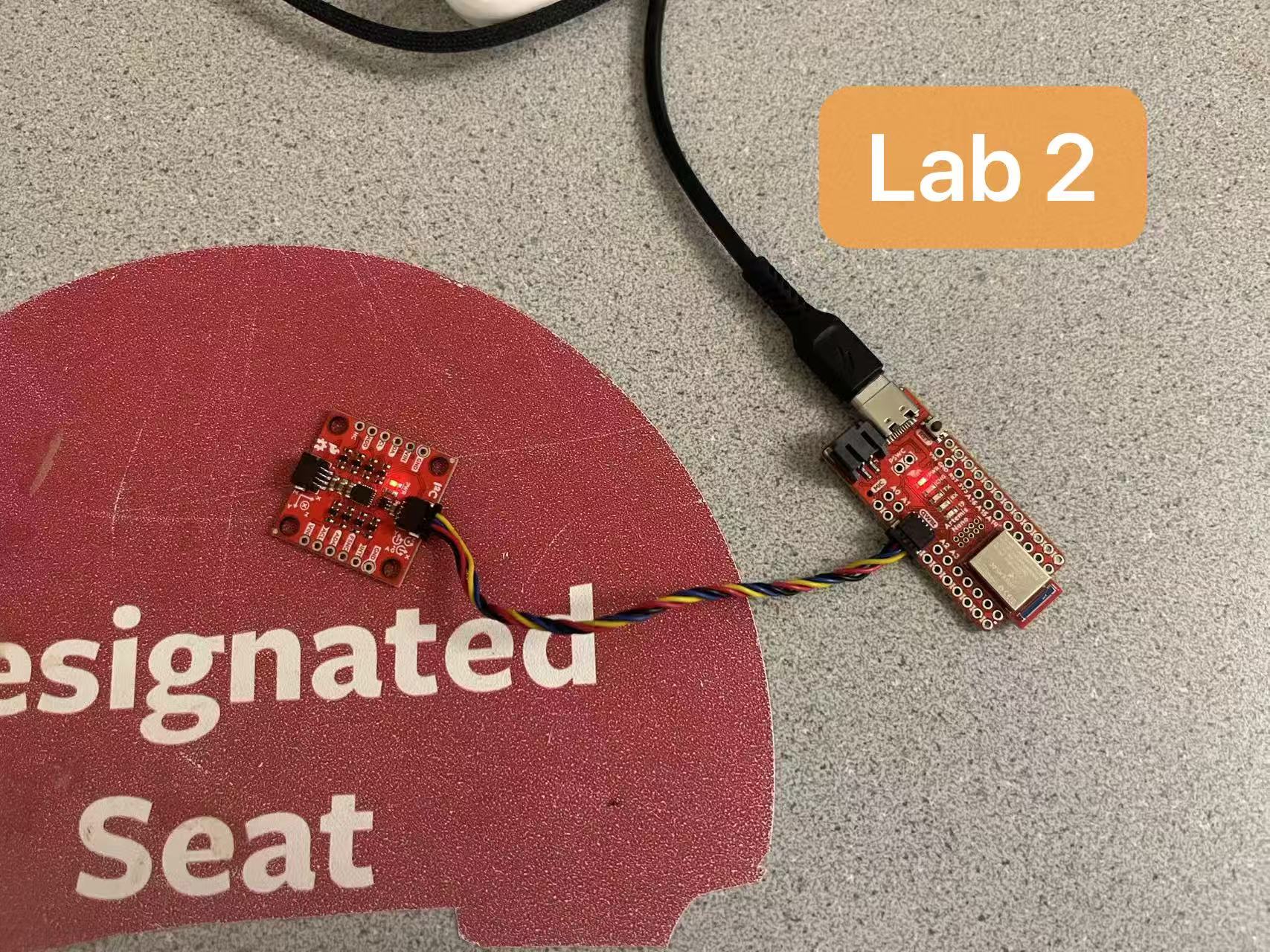
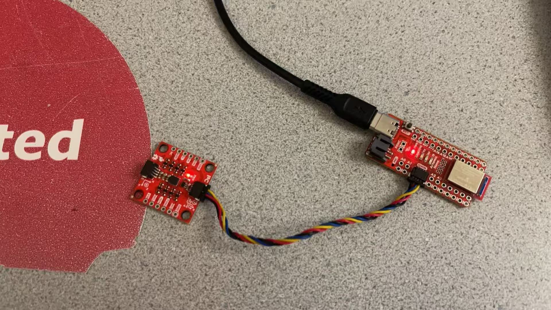
This experiment utilizes the SparkFun 9DoF IMU Breakout (ICM-20948), connected to the Artemis development board via an I²C interface. The Artemis board provides both power supply and communication.
To verify that the hardware connections and software environment were correctly configured,
the example program Example1_Basics from the SparkFun ICM-20948 Arduino library was executed.
The example outputs the following sensor data:
Accelerometer: Acc (mg) [ax, ay, az]
Gyroscope: Gyr (DPS) [gx, gy, gz]
Magnetometer: Mag (uT) [mx, my, mz]
Temperature: Tmp (°C)
AD0_VAL Definition
AD0_VAL represents the logic level of the AD0 pin on the ICM-20948 sensor and is used
to select the I2C communication address. Since the ADR jumper on the breakout board
is left unconnected by default, AD0_VAL was set to 1 in this experiment to match
the corresponding I2C address configuration.
Accelerometer and Gyroscope Data Characteristics
The accelerometer measures the combined effect of linear acceleration and gravity. When the
breakout board is stationary or slowly rotated, the measured values mainly reflect the gravity
components along each axis. For example, when the board is rotated by 180 degrees, an axis that
originally measured approximately +1 g will measure approximately −1 g, while the values on the
other axes change according to the board orientation. During rapid motion or acceleration, the
accelerometer readings exhibit noticeable fluctuations.
The gyroscope measures angular velocity. When the system is stationary, the output is close to
zero. During rotation or turning, clear angular velocity changes are observed. After motion
stops, the readings return close to zero, with only small amounts of noise and bias remaining.
Visual Indicator Verification
To verify that the program was running correctly on the Artemis, the onboard LED was used as a
visual indicator and configured to blink at a fixed time interval. Normal blinking of the LED
indicates that the program is executing successfully.
Accelerometer
Pitch / Roll Static Pose Verification
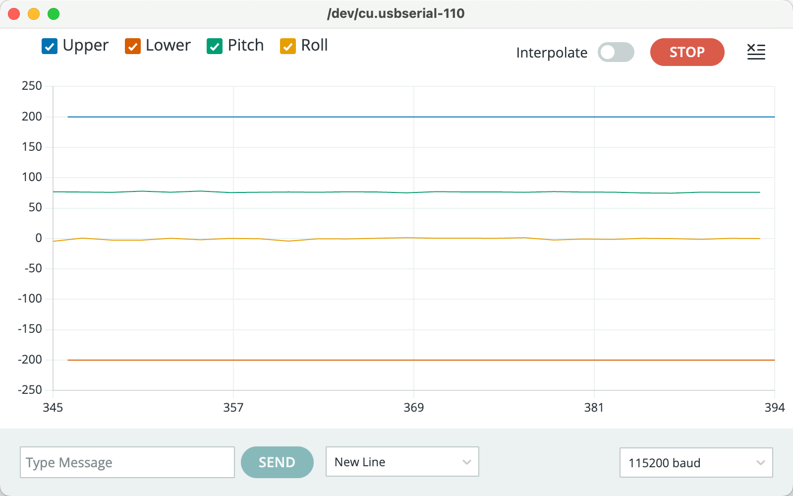
To evaluate the performance of the accelerometer in static orientation estimation,
the IMU was placed in four different static poses: Pitch = +90°, Roll = +90°,
Roll = −90°, and Pitch = −90°. For each configuration, the serial monitor output
was observed in real time to verify the corresponding accelerometer readings.
Figure 1. Pitch = +90°
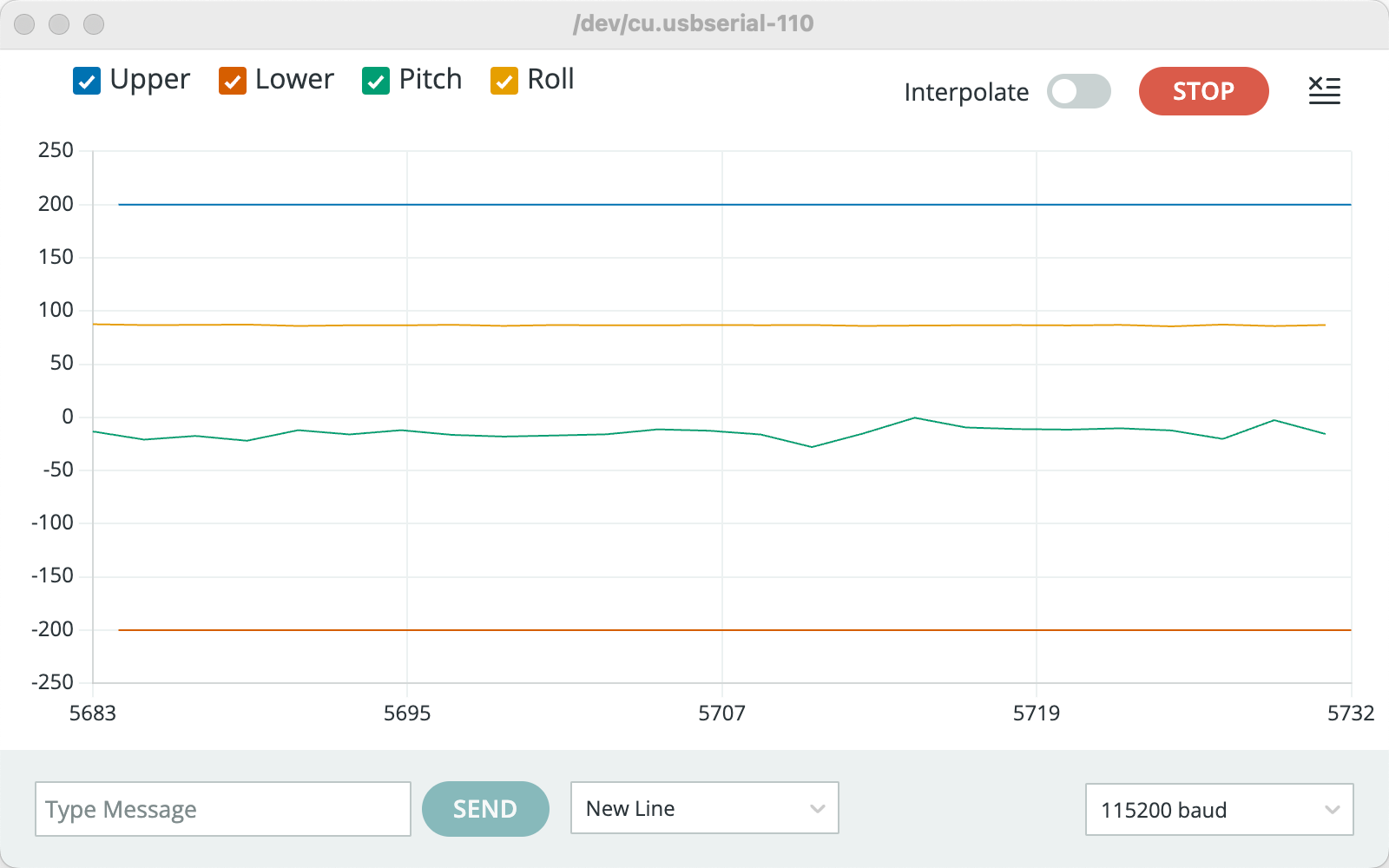
Figure 2. Roll = +90°
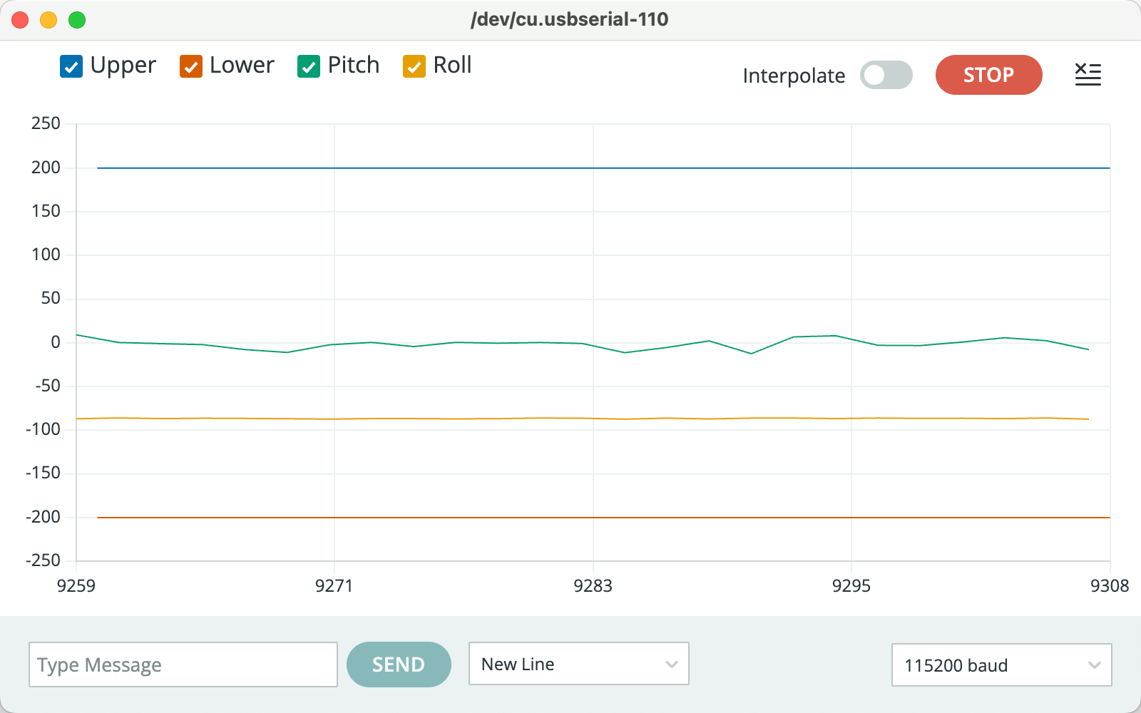
Figure 3. Roll = −90°
Figure 4. Pitch = −90°
Accelerometer Accuracy and Two-Point Calibration
To evaluate the accelerometer accuracy, a two-point calibration was performed on the Z-axis
using static measurements at +1g and −1g.
From the experimental data, the measured accelerometer outputs were:
m+ = 1024.36 mg,
m− = −988.54 mg
Ideally, these values should be +1000 mg and −1000 mg, respectively. The deviation indicates
the presence of sensor bias and scale error.
The calibrated Z-axis acceleration is then given by:
az,cal = ( az,raw − 17.91 ) × 0.9936
The results show that the accelerometer exhibits a small bias and a scale error of less than 1%.
After calibration, the measured acceleration closely matches the expected ±1g values, which is
sufficient for reliable pitch and roll estimation under static or low-dynamic conditions.
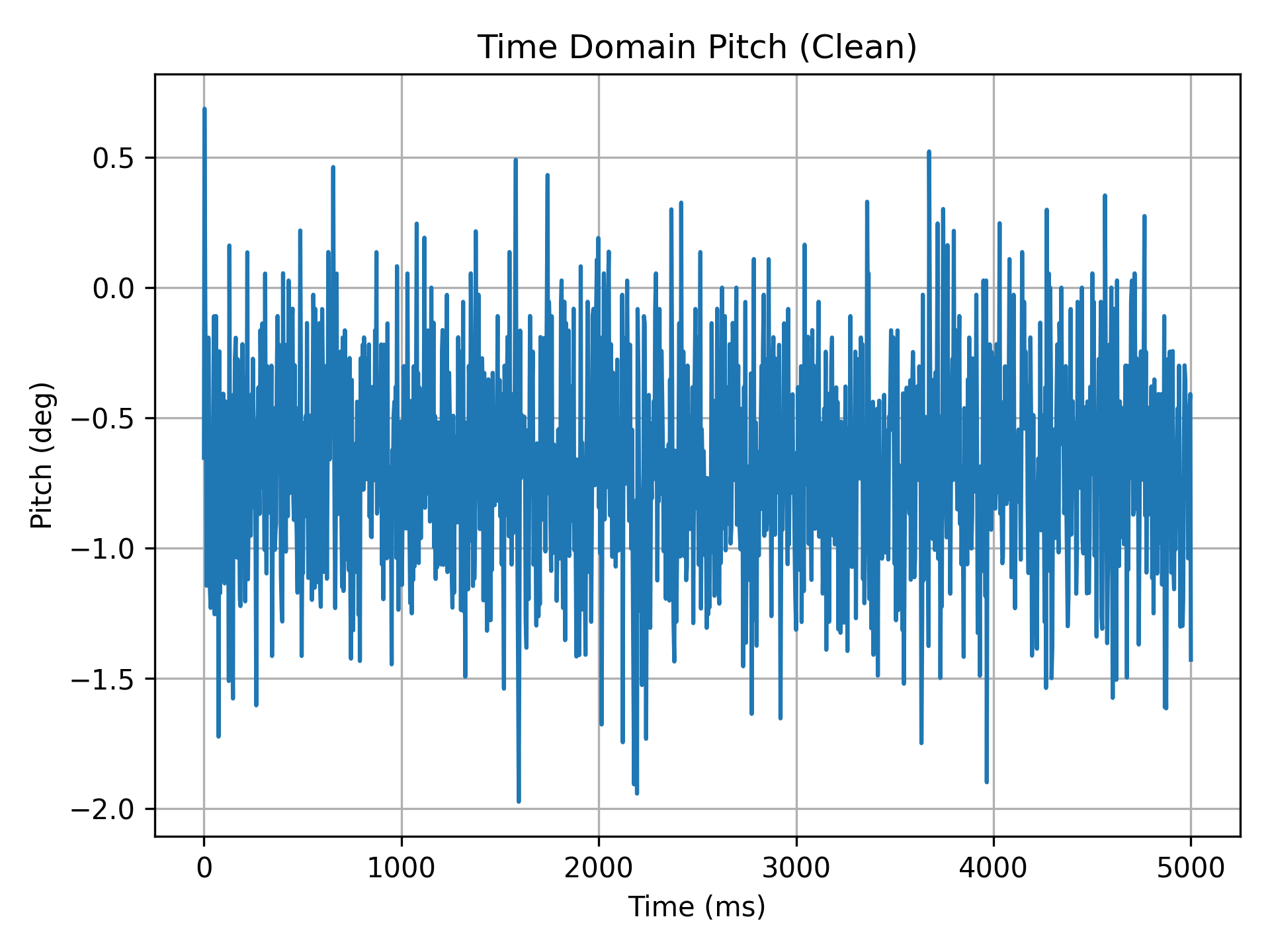
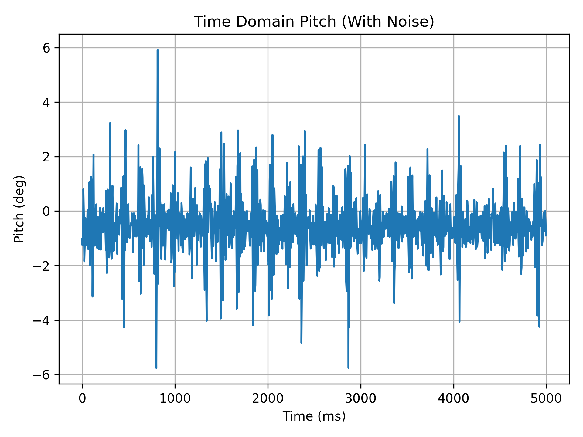
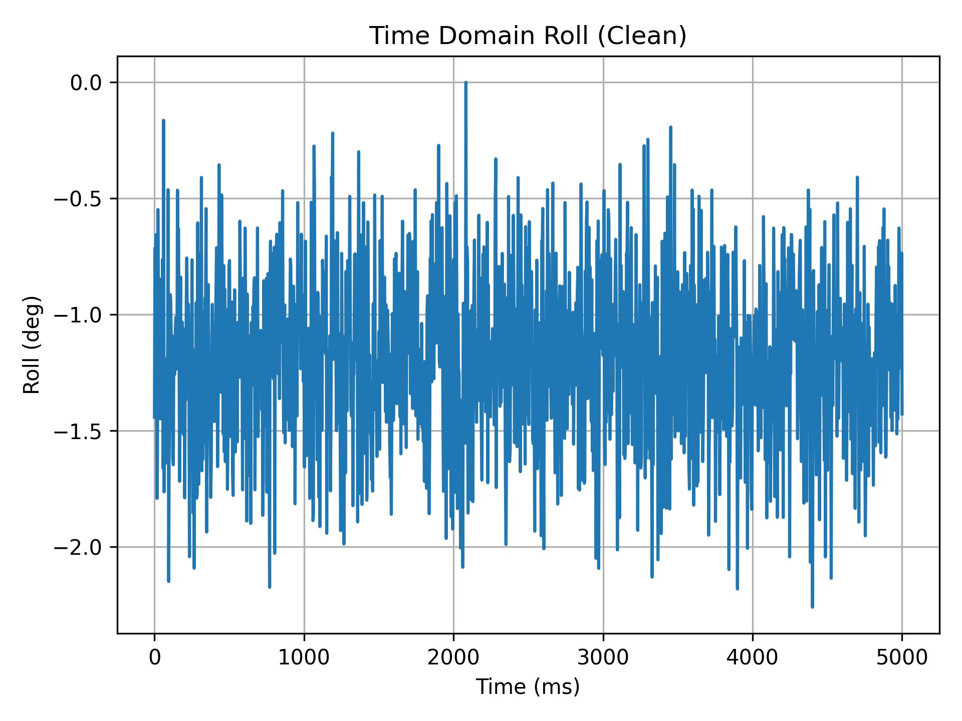
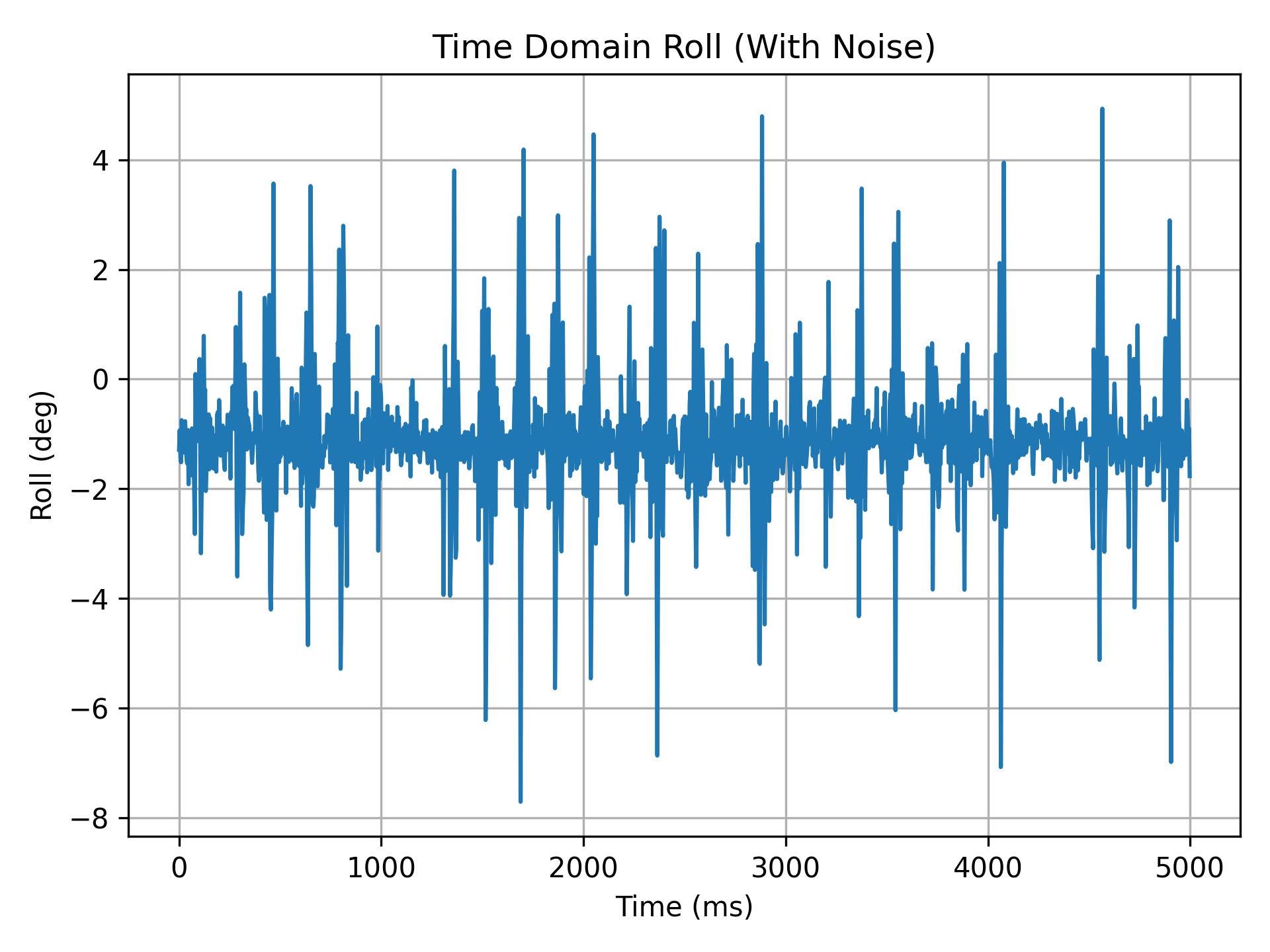
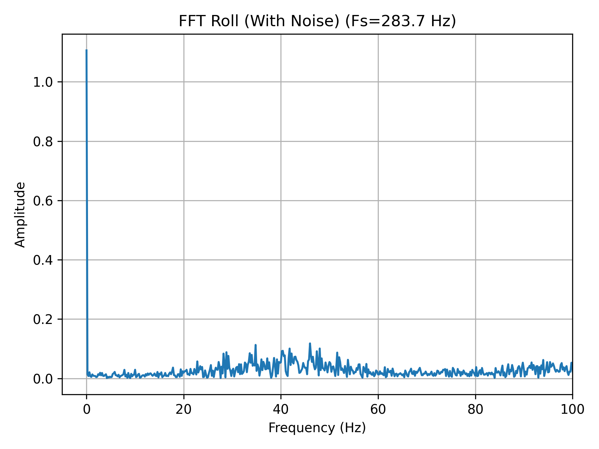
Accelerometer: Noise and Frequency-Domain Analysis (FFT)
To analyze the noise characteristics of the accelerometer data, time-domain and frequency-domain
(FFT) analyses were performed on the pitch and roll angle signals under two conditions:
static (clean) and with artificially introduced disturbances (with noise).
Figure 5. Time Domain Pitch (Clean)
Figure 6. Time Domain Pitch (With Noise)
Figure 7. Time Domain Roll (Clean)
Figure 8. Time Domain Roll (With Noise)
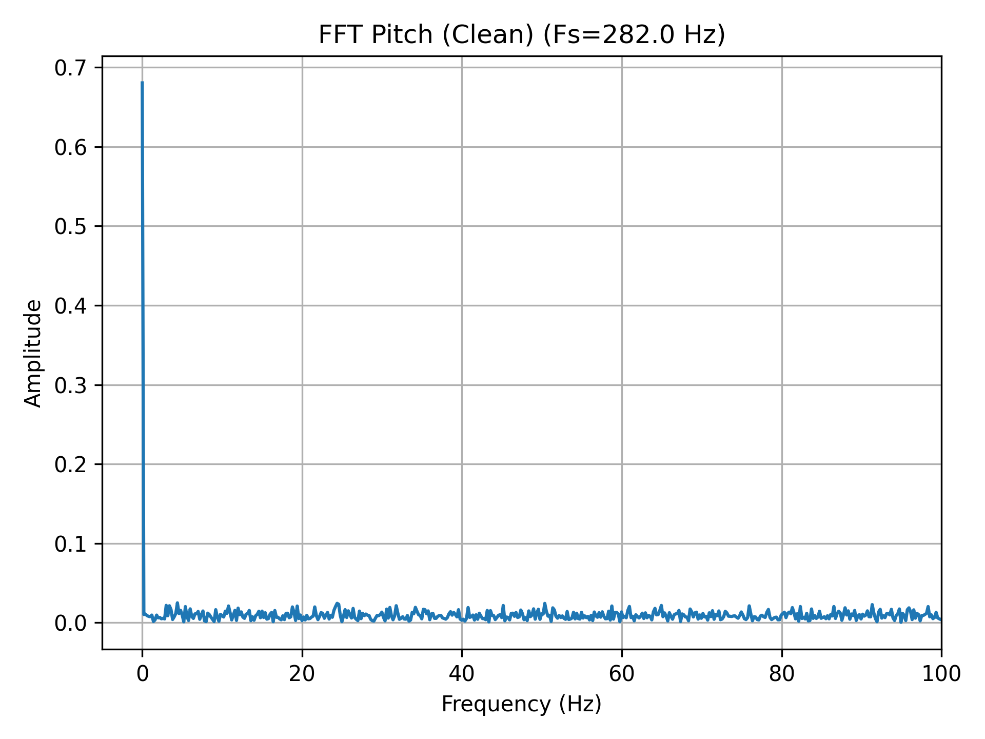
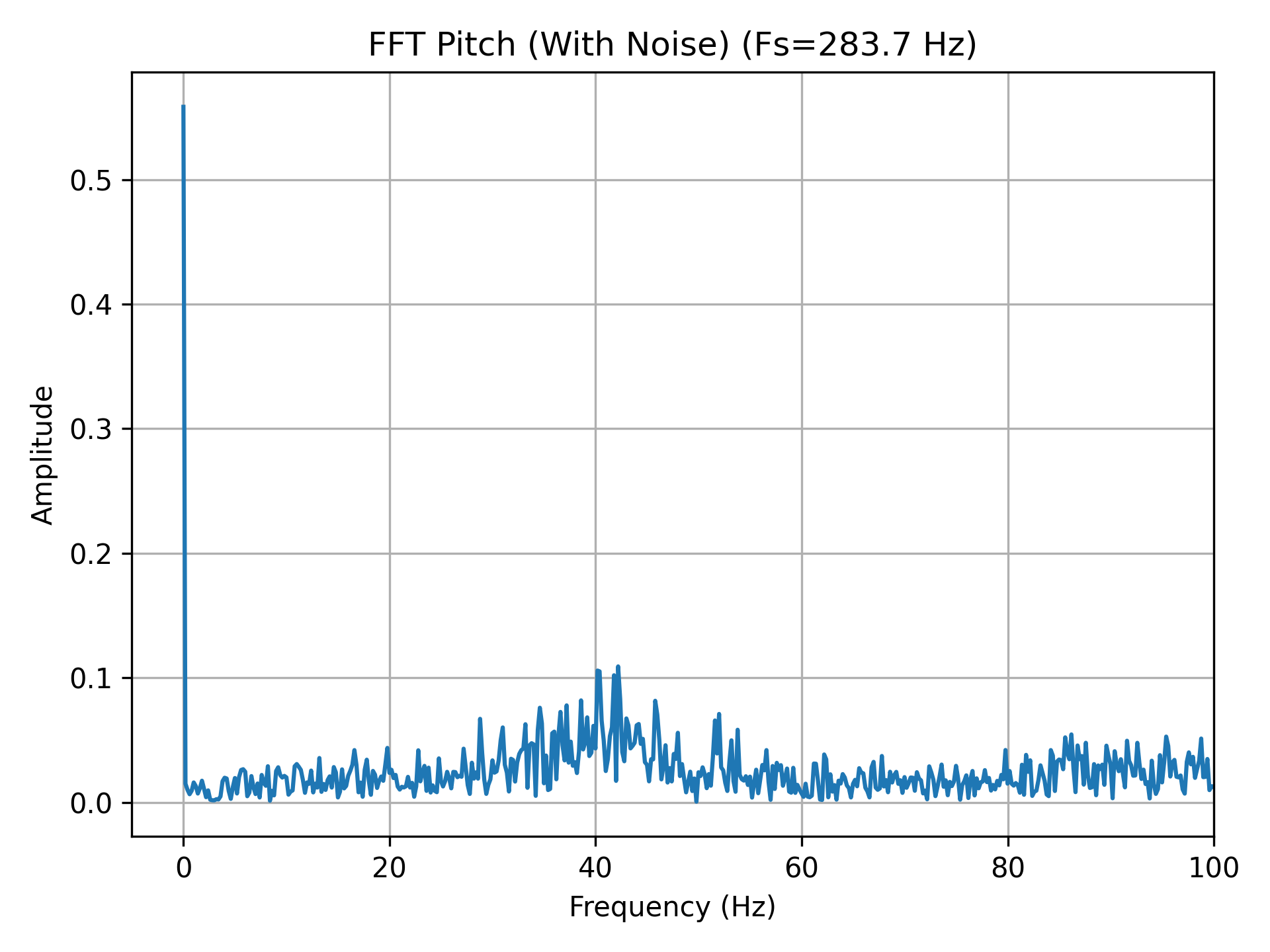
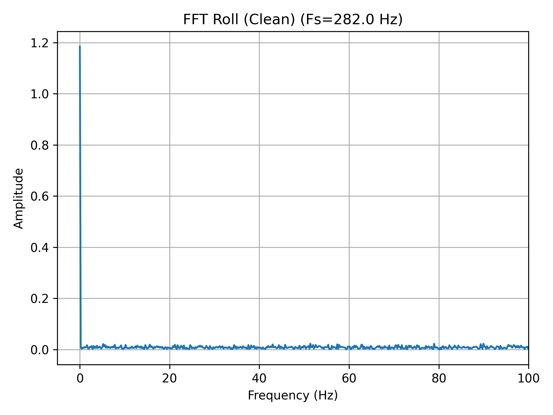
From the FFT results, it can be observed that the primary energy of both
pitch and roll is concentrated in the low-frequency region (around 3–4 Hz).
With \( f_s = 283 \,\text{Hz} \) and \( f_c = 3 \,\text{Hz} \),
\( \alpha \approx 0.062 \)
Figure 9. FFT Pitch (Clean)
Figure 10. FFT Pitch (With Noise)
Figure 11. FFT Roll (Clean)
Figure 12. FFT Roll (With Noise)
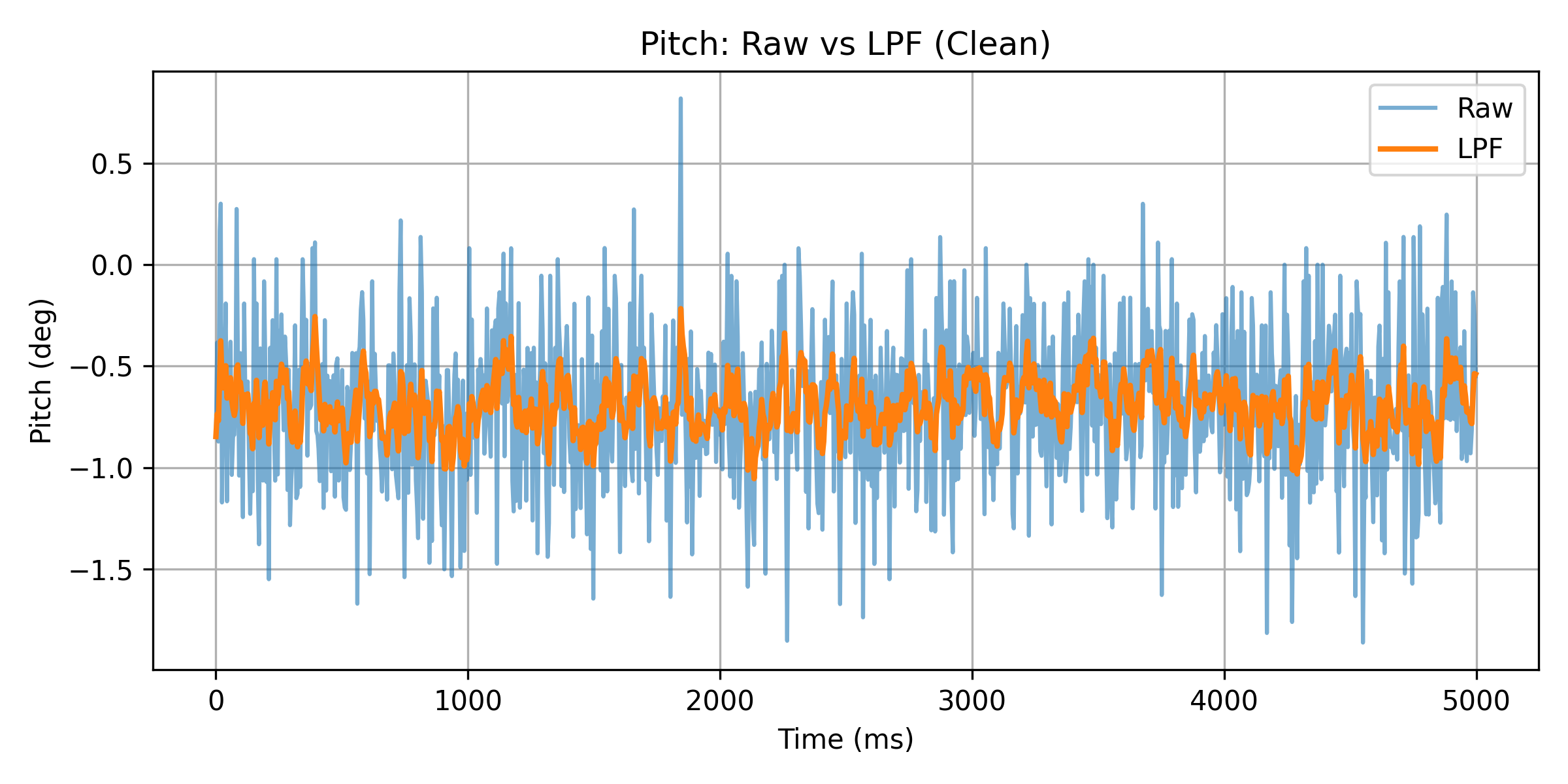
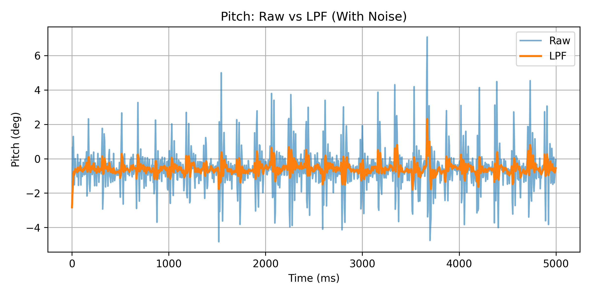
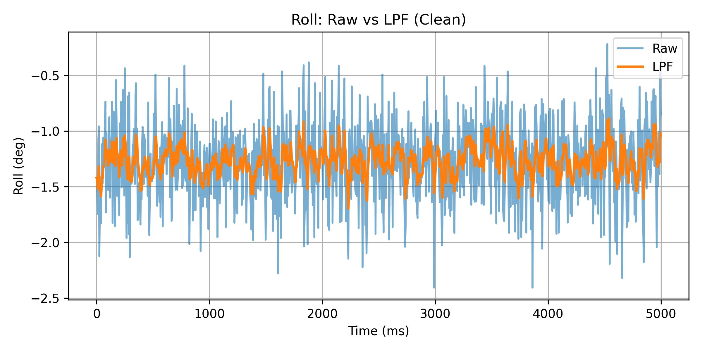
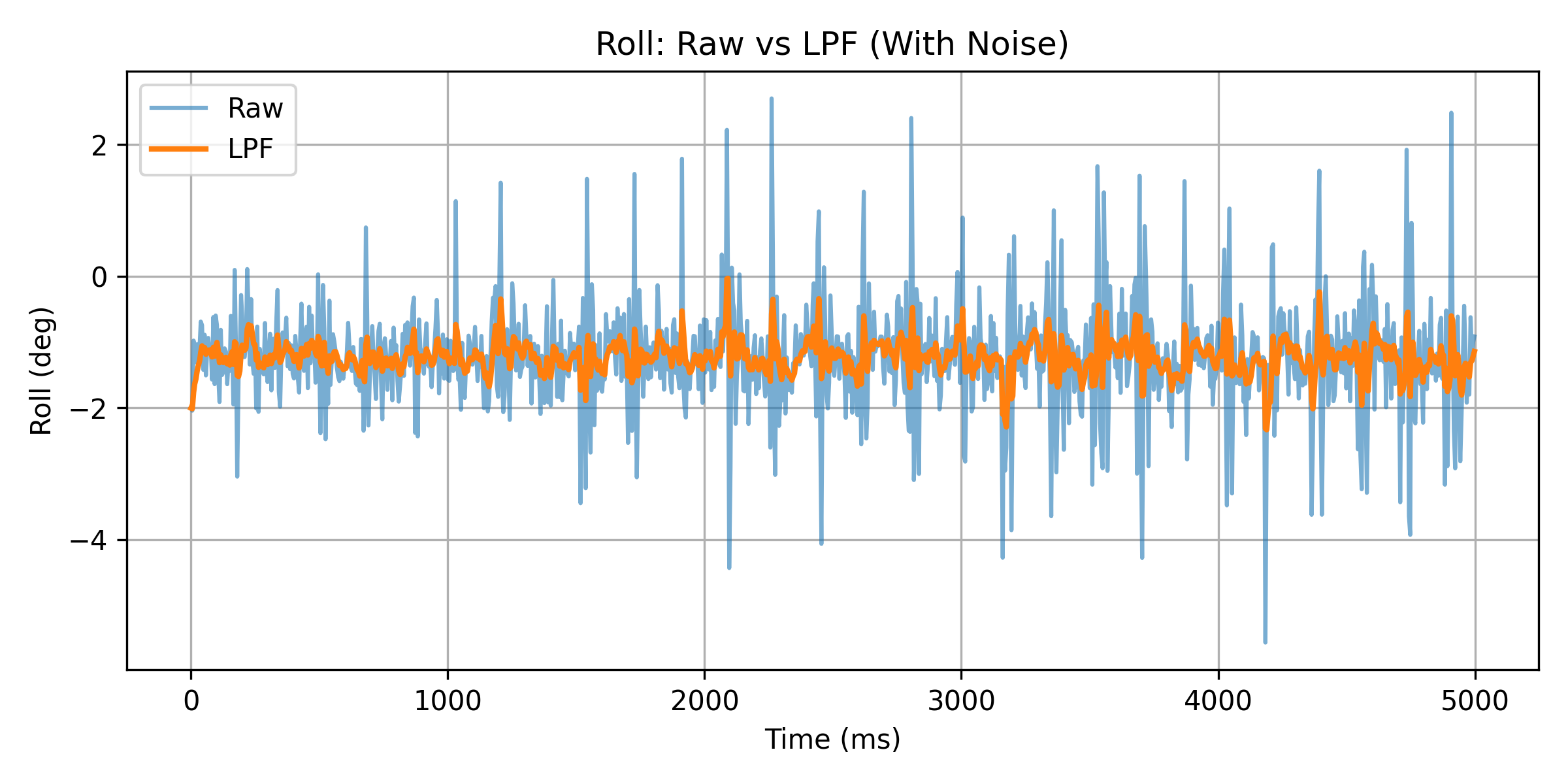
From the results, it can be observed that after applying the low-pass filter,
the high-frequency jitter in both the pitch and roll signals is significantly
reduced, resulting in much smoother curves. When noise is introduced, the
filtering effect becomes even more pronounced, with spikes and random
fluctuations being effectively suppressed. At the same time, the filtered
signals are still able to follow the overall trend of the original attitude
changes, indicating that the cutoff frequency is not set too low.
Figure 13. Pitch: Raw vs LPF (Clean)
Figure 14. Pitch: Raw vs LPF (With Noise)
Figure 15. Roll: Raw vs LPF (Clean)
Figure 16. Roll: Raw vs LPF (With Noise)
Lower cutoff frequency:
Produces a smoother output with better noise suppression. However, the
system response becomes slower, leading to noticeable lag during rapid
rotational motion.
Higher cutoff frequency:
Results in a faster response that can track rapid attitude changes more
easily, but introduces more high-frequency noise, causing increased
output fluctuations.
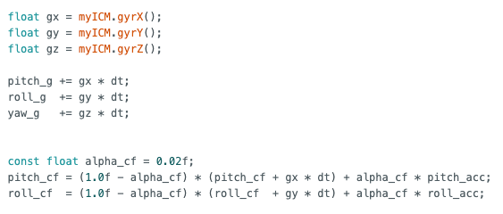
Gyroscope
The angle estimation is based on the integration model introduced in class:
Using the gyroscope angular velocity measurements, the pitch, roll, and yaw
angles are obtained through time integration.
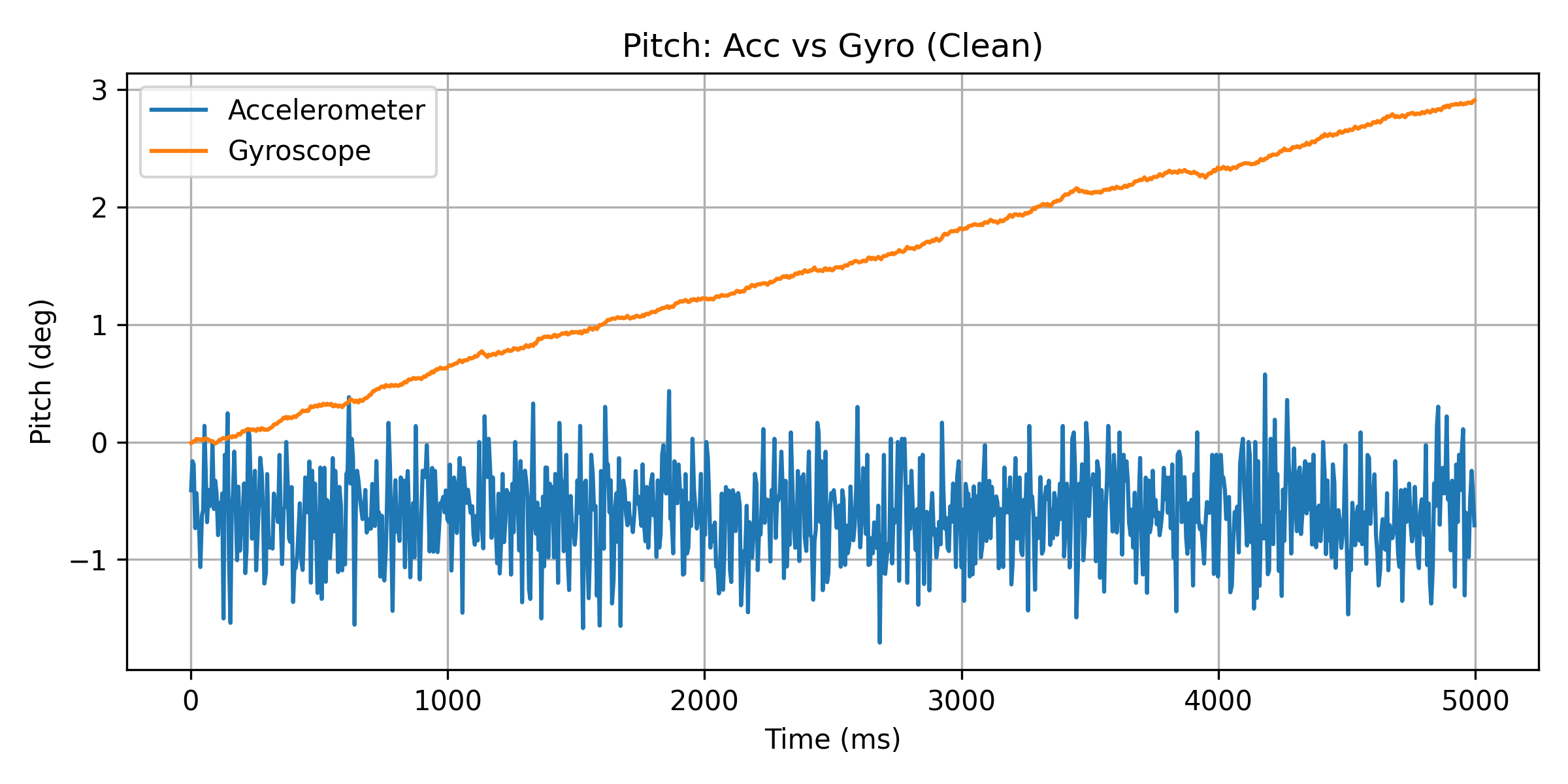
Figure 17. Pitch: Accelerometer vs Gyroscope (Clean)
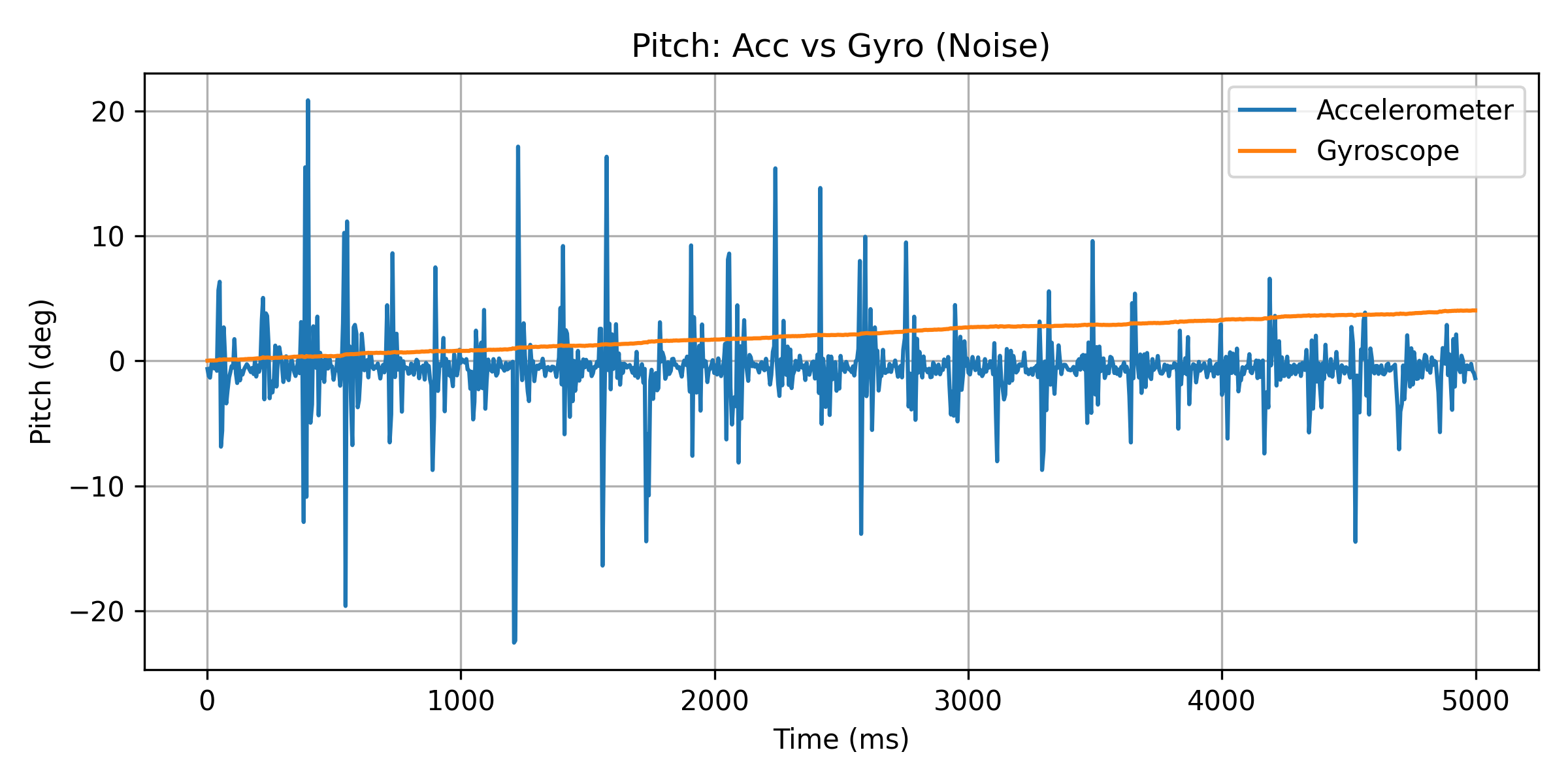
Figure 18. Pitch: Accelerometer vs Gyroscope (With Noise)
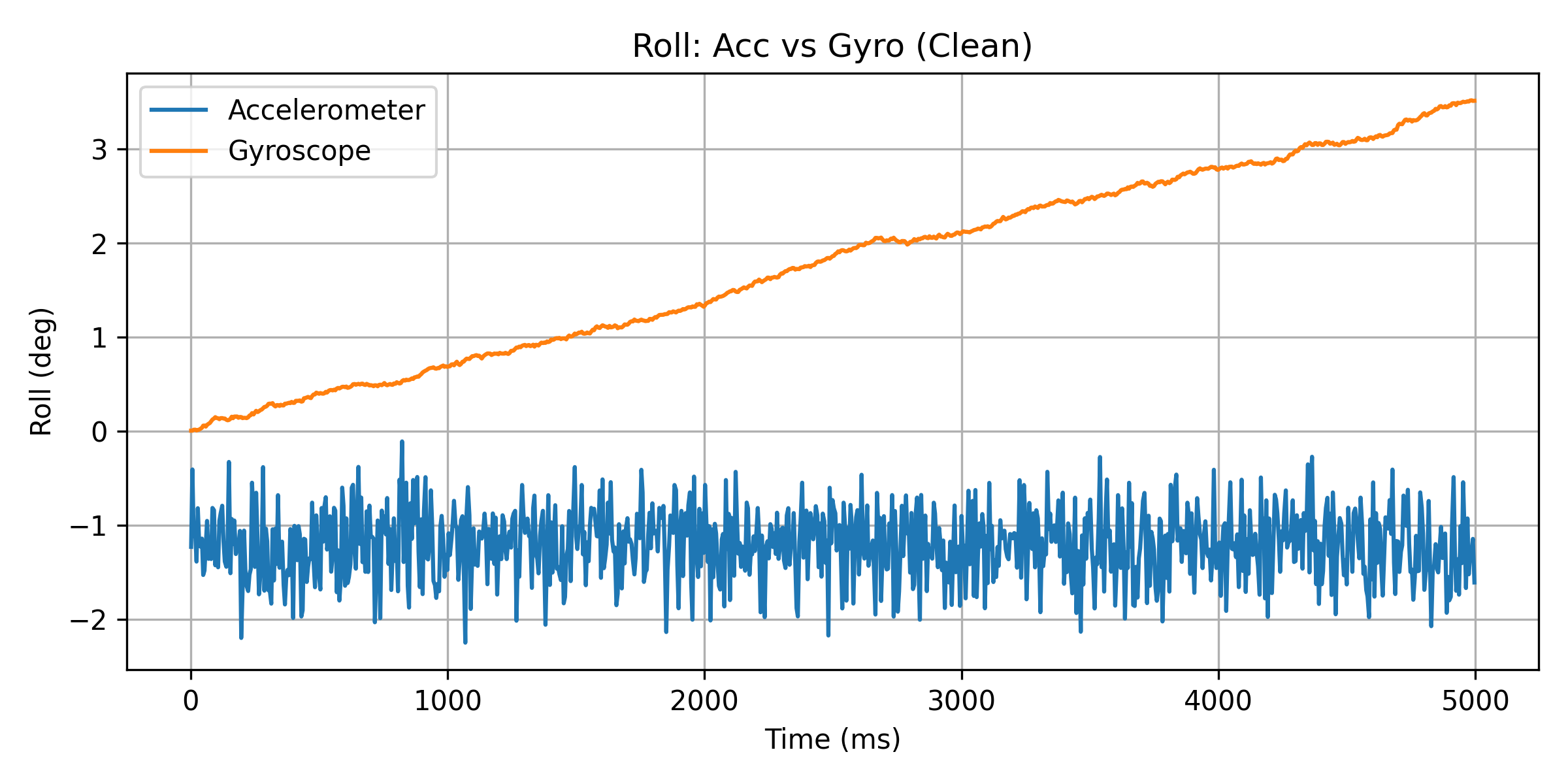
Figure 19. Roll: Accelerometer vs Gyroscope (Clean)
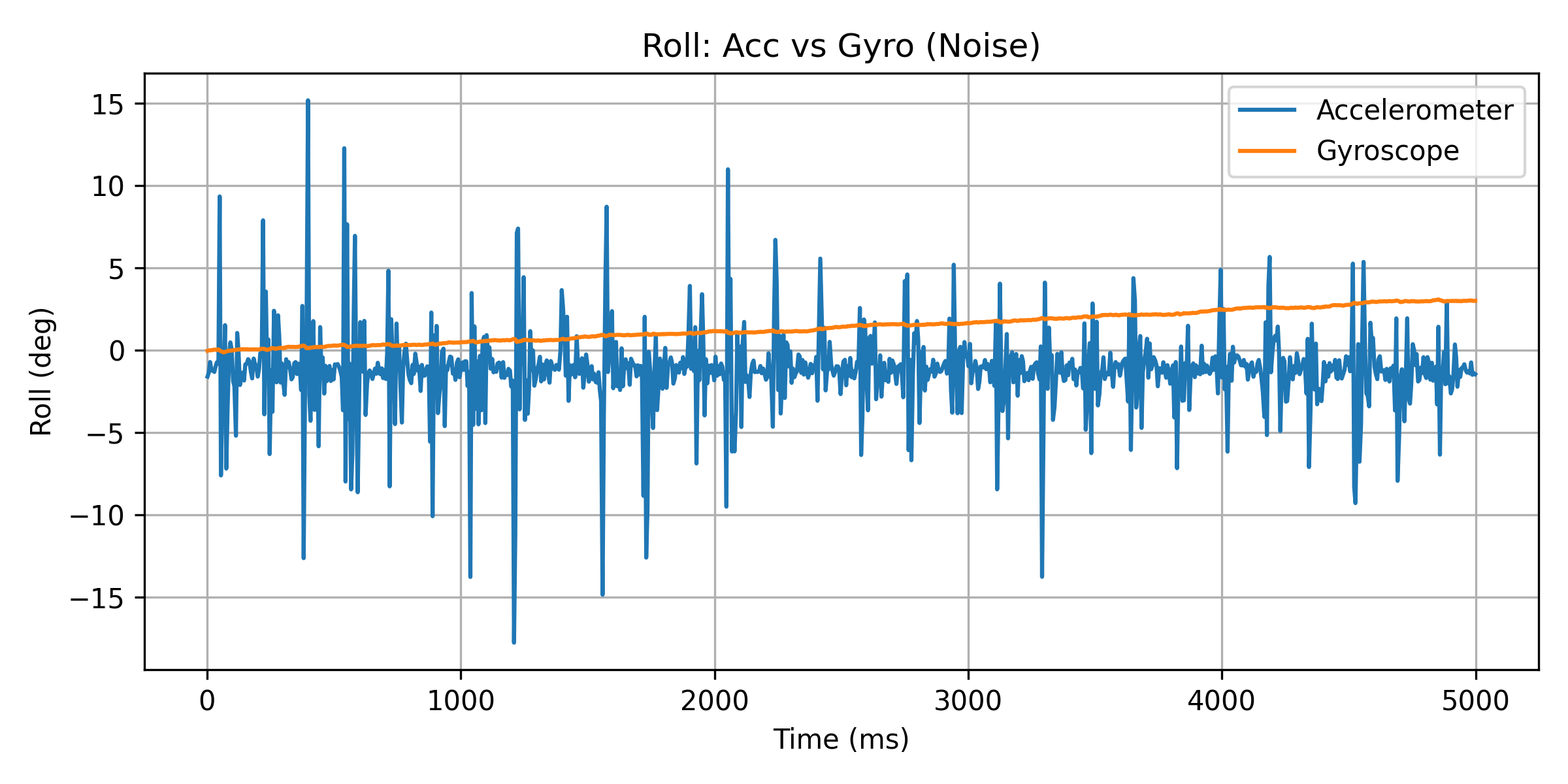
Figure 20. Roll: Accelerometer vs Gyroscope (With Noise)
The following differences can be observed from the results:
Accelerometer
Under static or low-dynamic conditions, pitch and roll can accurately
reflect the true orientation.
Highly sensitive to vibrations and external accelerations, resulting
in large noise and frequent spikes in the signal.
Exhibits significant angle fluctuations and reduced stability in
noisy environments.
Gyroscope
Produces smooth and continuous angle changes, with good response to
short-term motion.
Maintains relatively low noise levels in both clean and noisy
conditions.
Due to the accumulation of integration error, the estimated angle
gradually drifts over time, even when the system is stationary.
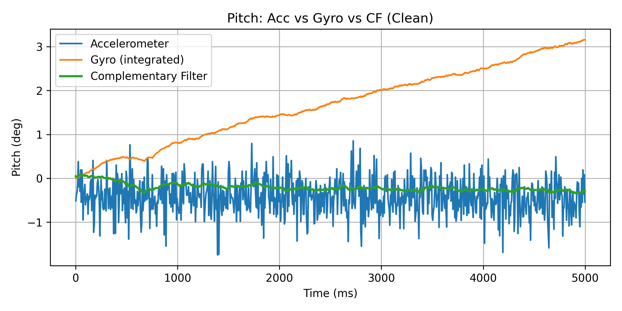
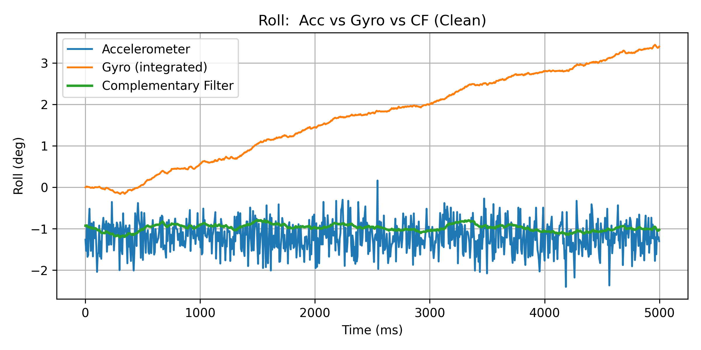
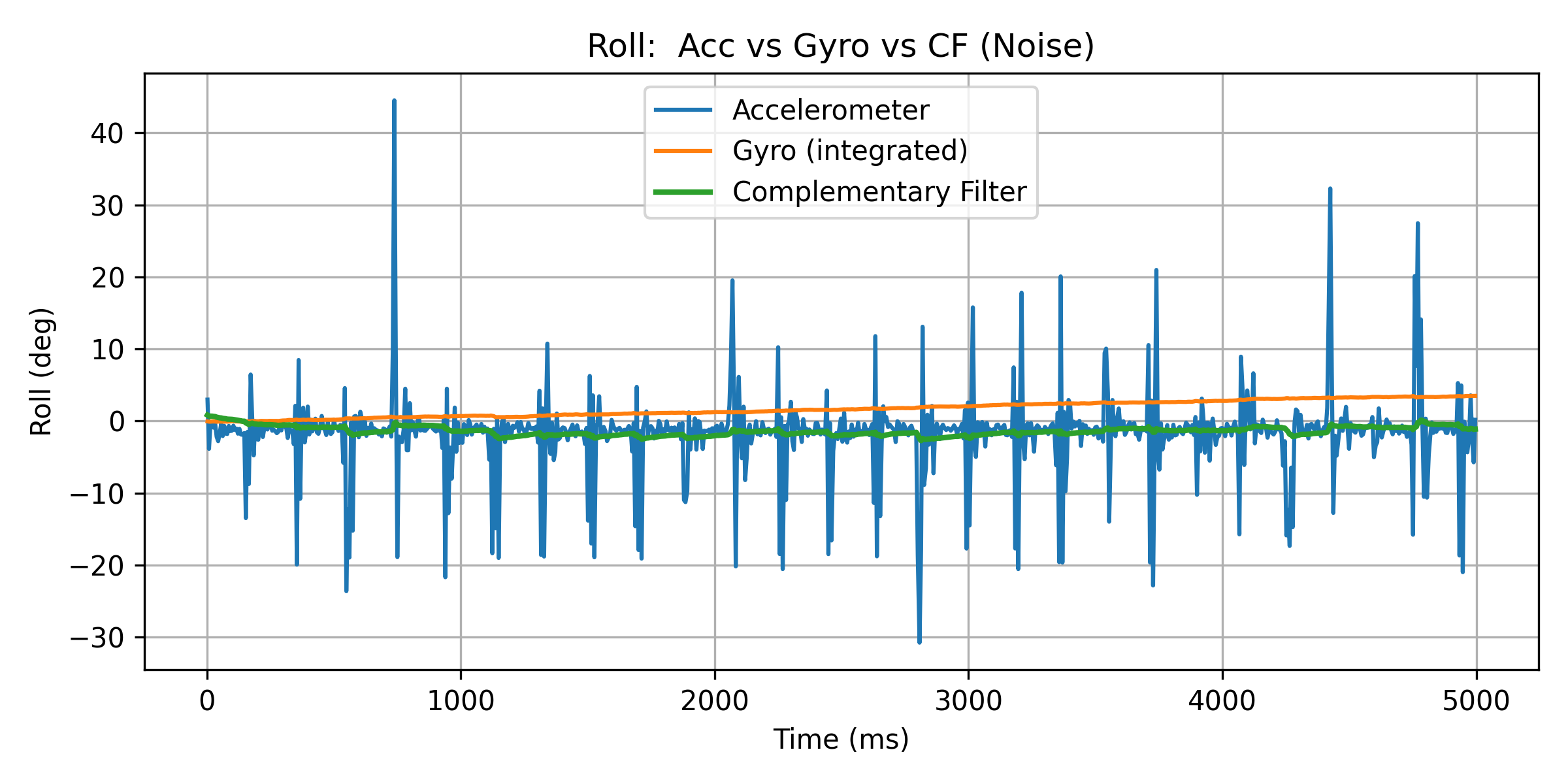
In this experiment, the complementary filter provided in the lecture was adopted
to fuse the gyroscope-integrated angle with the accelerometer-based attitude angle:
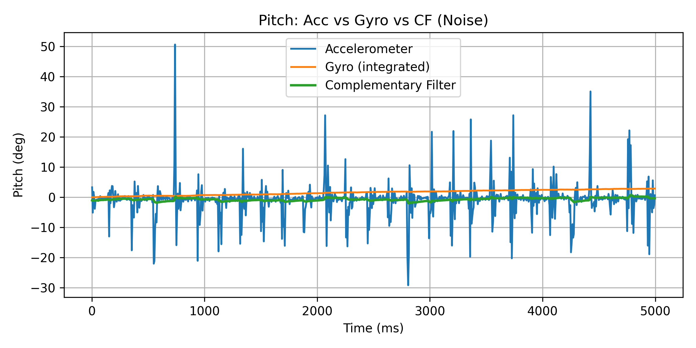
When only the accelerometer is used, both pitch and roll angles exhibit a large
number of spikes under noisy conditions, indicating high sensitivity to instantaneous
acceleration and external vibrations.
When only the gyroscope integration is used, the output is relatively smooth;
however, significant drift accumulates over time, causing the estimated angle
to gradually deviate from the true value.
By contrast, the complementary filter provides stable and smooth outputs in both
clean and noisy scenarios. High-frequency noise from the accelerometer is effectively
suppressed, while the long-term drift of the gyroscope is significantly corrected.
Figure 21. Pitch: Acc vs Gyro vs CF (Clean)
Figure 22. Pitch: Acc vs Gyro vs CF (With Noise)
Figure 23. Roll: Acc vs Gyro vs CF (Clean)
Figure 24. Roll: Acc vs Gyro vs CF (With Noise)
Sample Data
1) Speed of Sampling
To maximize the data acquisition rate, the main loop avoids blocking or
waiting for the IMU. Instead, each loop iteration checks whether new IMU
data are available (data ready). Data are read and stored only when new
samples are detected.
All debugging-related delay() and
Serial.print() statements were removed to prevent serial
communication from becoming a performance bottleneck.
From a 5-second sampling window, len(t) = 1608,
corresponding to an average sampling rate of:
fs ≈ 1608 / 5 ≈ 322 Hz (≈ 3.1 ms per sample)
Since the main loop runs faster than the IMU data update rate, this
polling-based approach (“check data ready + log when available”) maximizes
effective sampling while avoiding repeated reads of the same data frame.
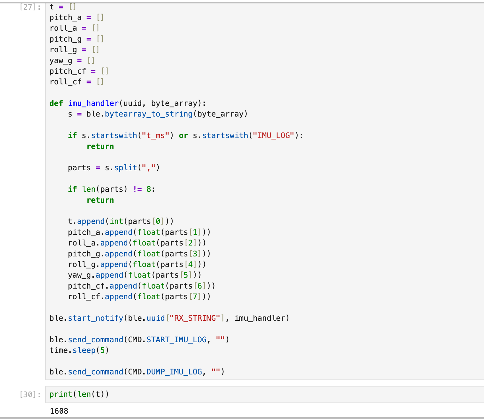
2) Time-Stamped Data Storage
IMU data were stored in time-stamped arrays. Each record contains eight
fields:
The host computer receives the data via BLE notifications, parses the
comma-separated values, and appends them to the corresponding arrays.
3) Storage Structure and Data Type Selection (Design Choices)
Storage structure:
A parallel multi-array design was adopted, where each variable is stored in
an independent array. This structure simplifies post-processing in Python,
such as individual plotting, FFT analysis, and filter comparison, while
avoiding the parsing and indexing complexity associated with a single large
structured array.
Data types:
Time stamps are stored as int values (millisecond resolution),
while attitude angles are stored as float. This choice provides
a good balance between numerical precision and memory usage.
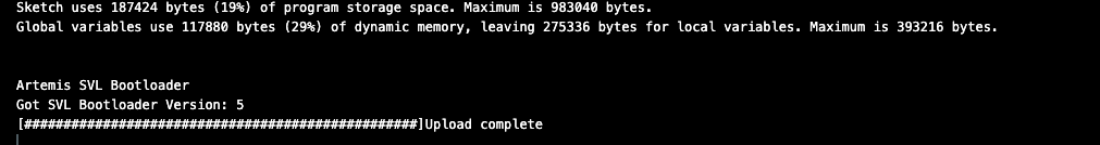
Based on the compiler output, the program uses approximately
187,424 bytes (19%) of Flash memory, and global variables
occupy about 117,880 bytes (29%) of RAM. This leaves
approximately 275,336 bytes of free RAM available for data
logging. With a data format consisting of one timestamp (int)
and multiple float values per sample, storing several seconds
of IMU data in memory is feasible.
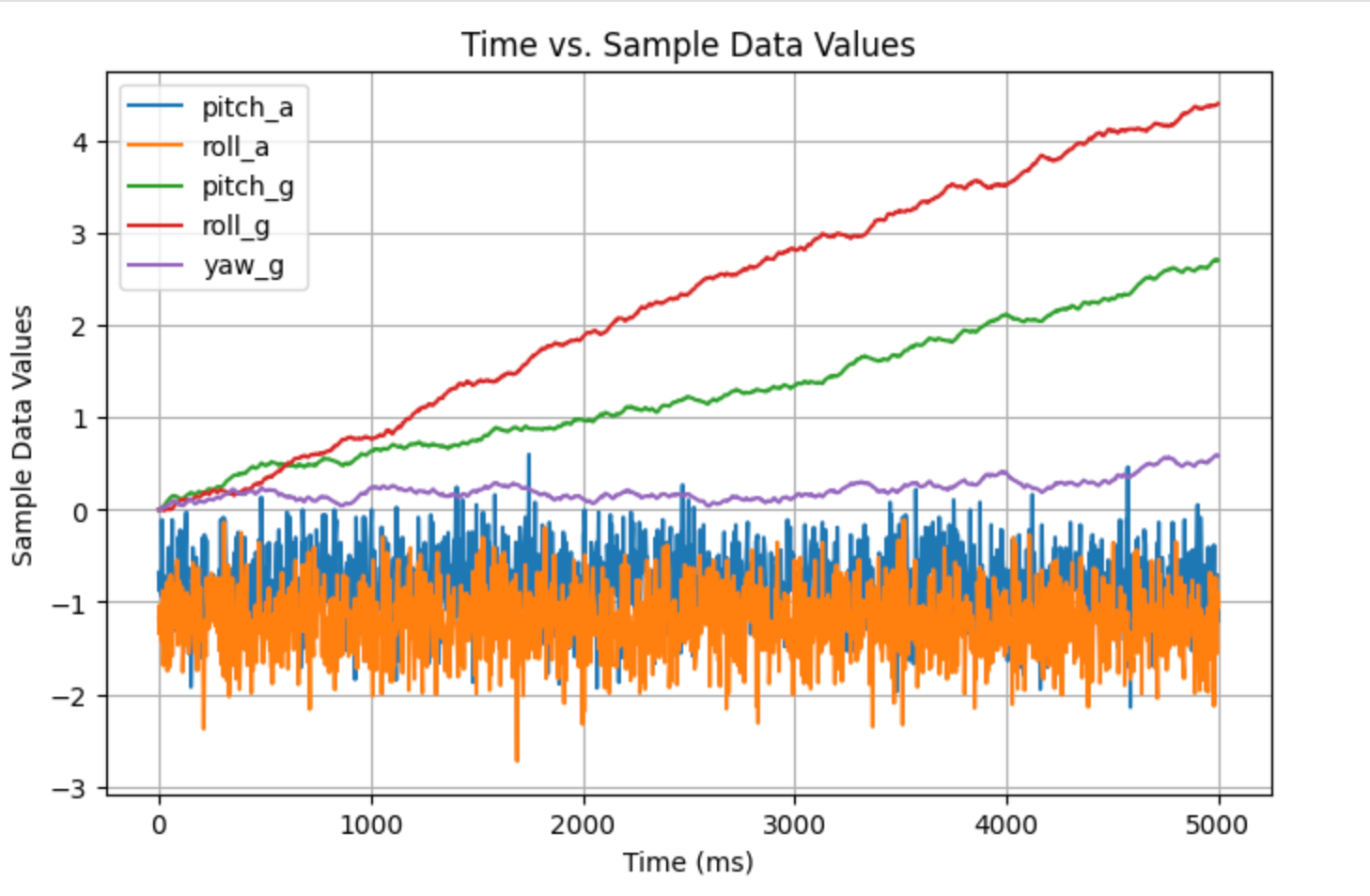
4) Five-Second Data Collection and BLE Transmission (5s over BLE)
The host computer sends the START_IMU_LOG command to initiate
data recording. After a 5-second acquisition window, the
DUMP_IMU_LOG command is issued to request data transmission.
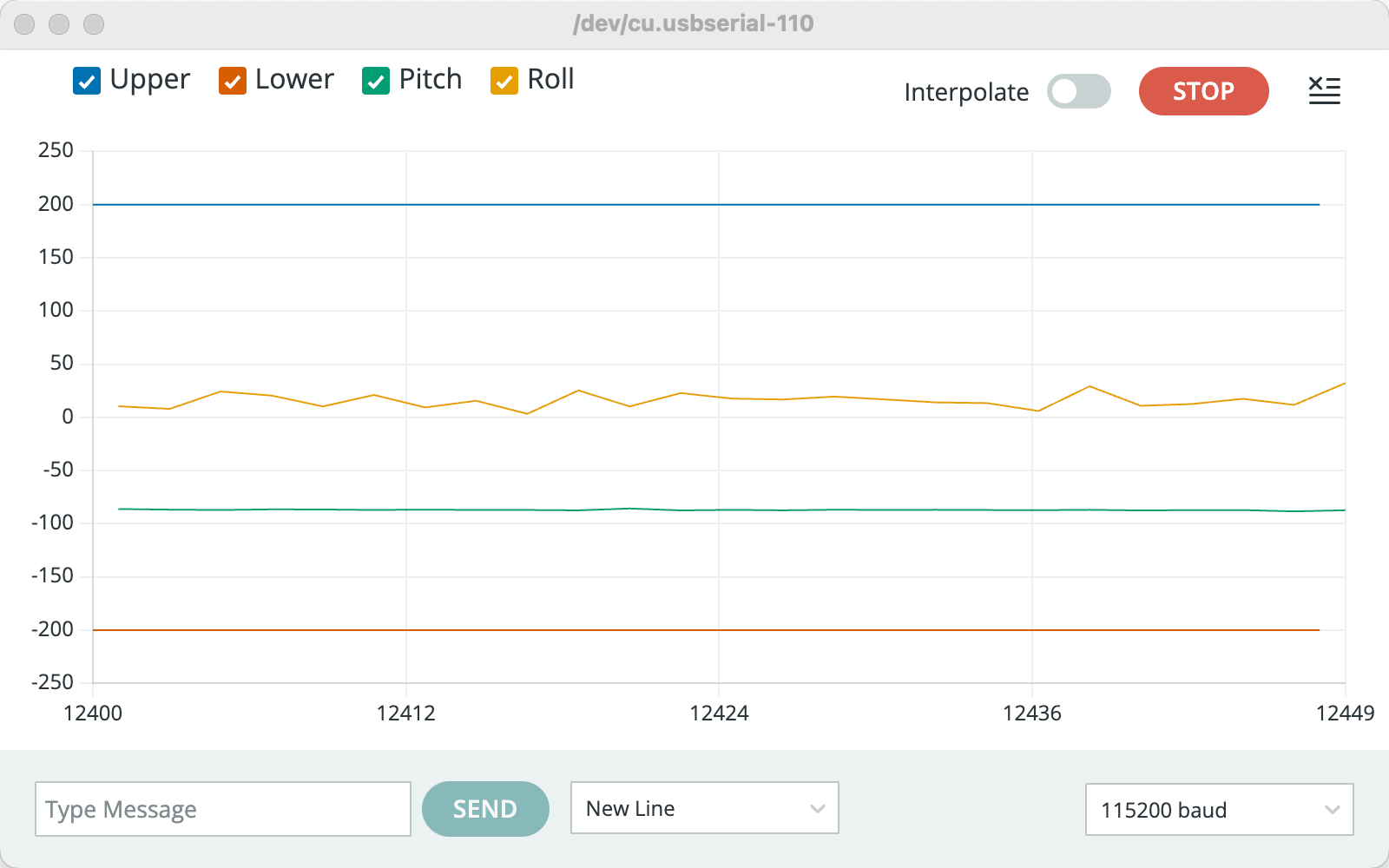
A total of 1608 time-stamped IMU samples were successfully
received. The resulting plots span the time range from 0 to 5000 ms
(Time vs. Sample Data Values), demonstrating that the system can reliably
complete the full pipeline of data acquisition, buffering, BLE transmission,
host-side parsing, and visualization within a 5-second window.
Record a stunt!
When the car impacts a wall at high speed, it rebounds and flips over, yet remains functional and can continue to operate.
Lab 3: Time of Flight Sensors
Prelab
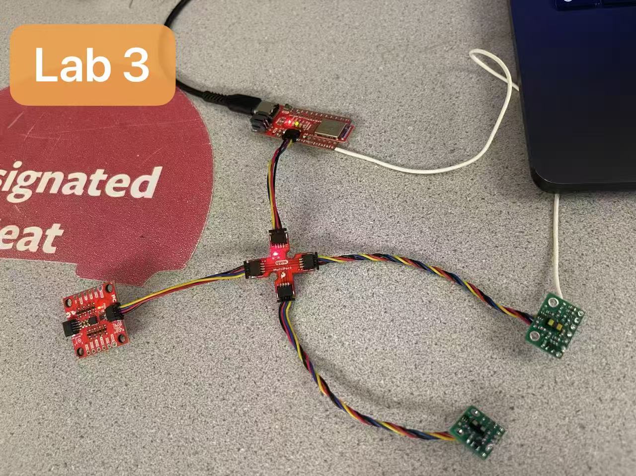
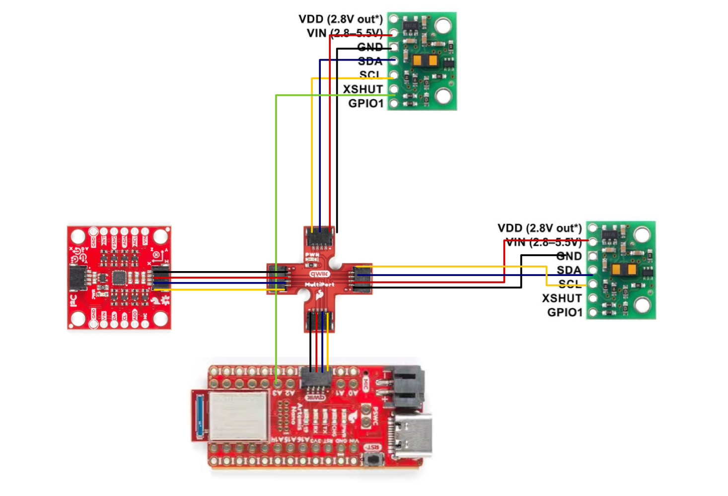
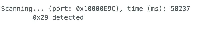
This experiment utilizes the VL53L1X Time-of-Flight (ToF) distance sensor, communicating with the Arduino via I2C. The default I2C address of the VL53L1X is typically displayed as 0x29 (7-bit). Since both VL53L1X sensors share the same factory default address, connecting them directly to the same I2C bus would cause an address conflict. Therefore, differentiation is required during the initialization phase. I employ a method combining XSHUT control with address modification: At startup, pull one sensor low via XSHUT to keep it disabled. Initialize only the other sensor and modify its I2C address to a new value (e.g., 0x30). Subsequently release XSHUT to enable the second sensor, allowing both sensors to coexist with distinct addresses and perform parallel sampling.
Wiring is shown in the figure: The Artemis connects to the Qwiic MultiPort via QWIIC (I2C). The IMU shares SDA/SCL, VIN, and GND with both VL53L1X sensors. To enable individual power-up activation and address assignment, I additionally connected one ToF sensor's XSHUT pin to an Artemis GPIO (green wire in the diagram). This allows selective disabling/enabling of that sensor during initialization.
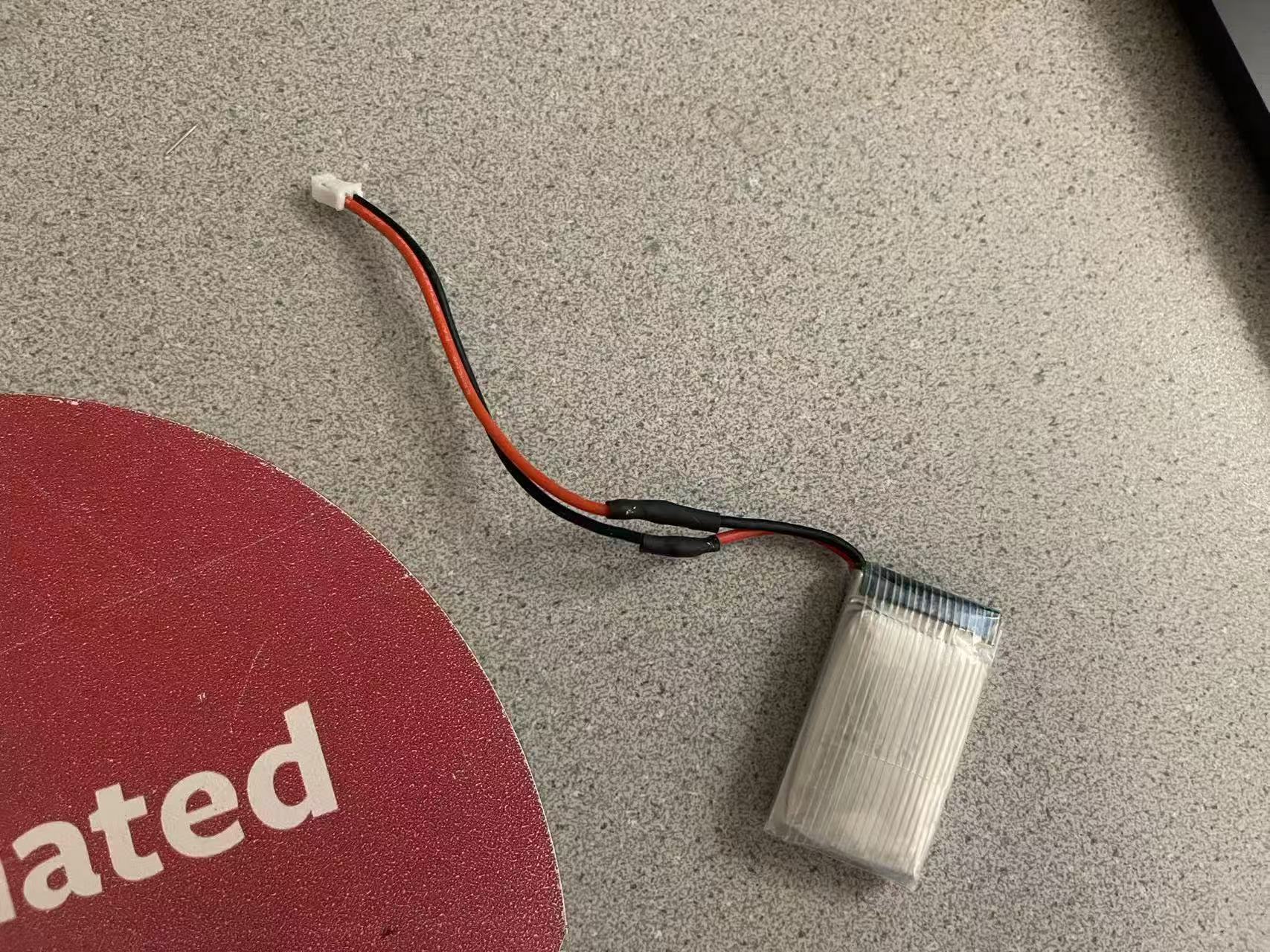
Task 1: Battery
After cutting the battery wires, I soldered them to the JST connectors
and insulated each solder joint with heat shrink tubing. To prevent
short circuits during operation, I cut only one wire at a time,
soldering and insulating it before proceeding to the next. This ensured
that the positive and negative terminals were never exposed and in
contact simultaneously.
Additionally, when verifying polarity, I discovered that the actual
positive and negative terminals of the battery wires were reversed from
their color markings. Therefore, the final connections were made by
connecting the red wire to the black terminal and the black wire to the
red terminal. This ensures the battery's positive terminal connects to
the Artemis's positive terminal and the negative terminal connects to
the Artemis's negative terminal.
As you can see in the video, when Artemis is powered by its battery, it can still communicate with the computer via Bluetooth.
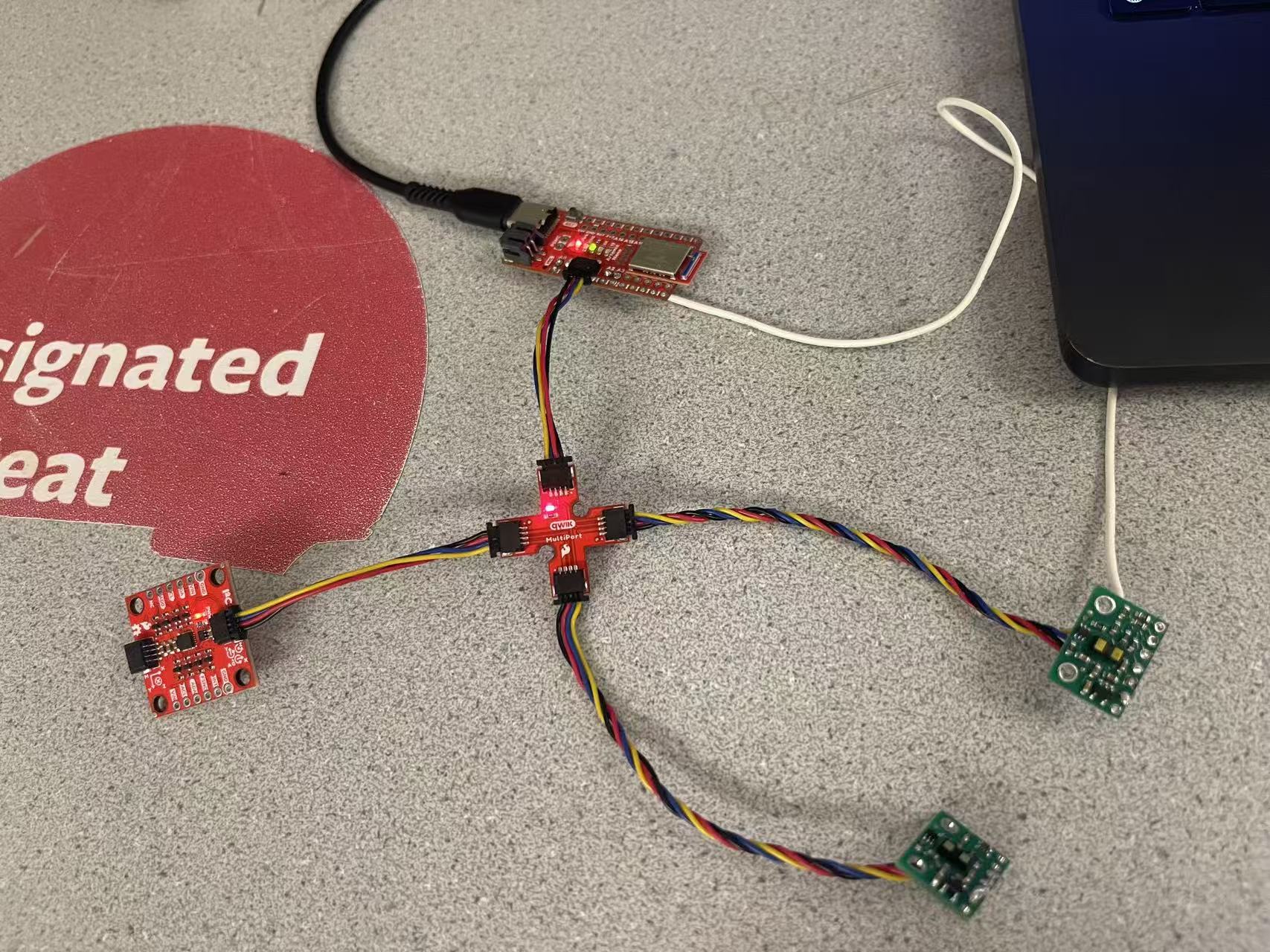
Task 2: Connections
As shown in the diagram above, I connected two ToF sensors to the Artemis
board via a QWIIC MultiPort splitter board. To facilitate future
installation of the ToF sensors at designated locations on the vehicle
body and simplify cable routing, I selected longer QWIIC cables for both
ToF sensors. For wire color assignment, I connected the blue wire to SDA
and the yellow wire to SCL, while the remaining power and ground wires
were connected according to QWIIC standards.
Additionally, to enable independent activation and address assignment
during dual ToF initialization, I soldered an extra wire to bring out
the XSHUT pin from one ToF sensor and connect it to pin A3 on the Artemis
board. This allows for individual shutdown/activation control of that
sensor within the program.
Task 3: I2C Channel
When scanning the I2C bus to confirm the sensor address, the datasheet
specifies an address of 0x52, but when I used Arduino's Example05_wire_I2C
to scan, the address detected was 0x29. These appear different but
actually represent the same address: 0x52 is the 8-bit address format
including the least significant R/W bit, while scanners typically display
the 7-bit address after removing the R/W bit. Therefore, removing the
least significant R/W bit from 0x52 (equivalent to shifting right by one
bit) yields 0x29, matching the scan result. This confirms the sensor
address is as expected.
Task 4: Sensor Configurations
The VL53L1X offers three ranging modes: Short, Medium, and Long, with
maximum ranges of approximately 1.3 m, 3 m, and 4 m respectively. Long
mode provides the greatest distance but tends to be less stable in strong
ambient light or with low-reflectivity targets, and typically has a lower
refresh rate. Medium mode represents a compromise. Short mode, while
offering the shortest range, delivers more stable readings at close
distances, better interference resistance, and facilitates higher sampling
frequencies.
Therefore, I ultimately selected short mode. The primary reasons are its
more reliable readings at close range and its suitability for increasing
sampling frequency. This enables a more responsive control loop, aligning
better with the final robot's application scenario of indoor close-range
navigation.
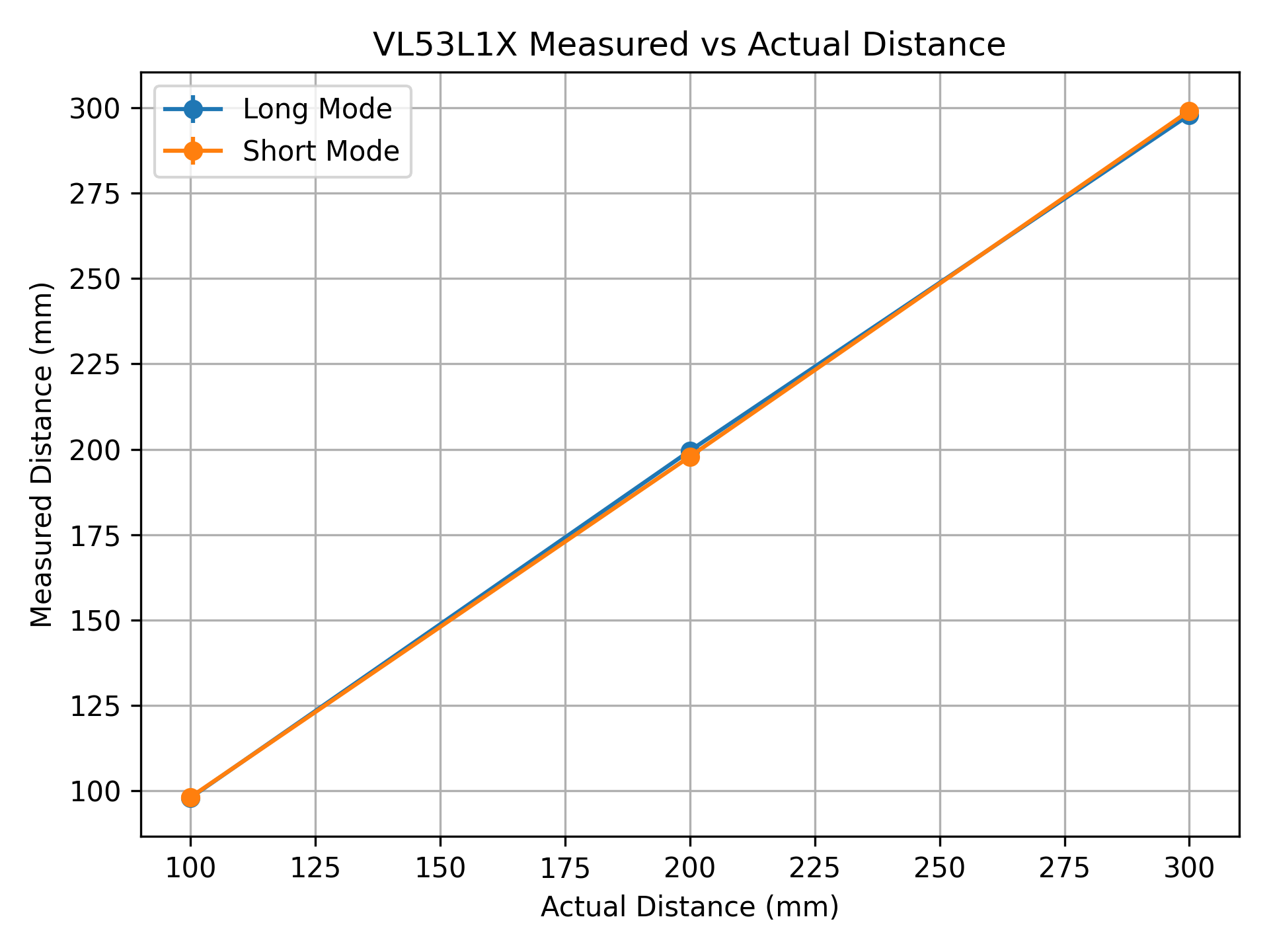
I conducted simple calibration tests in both Short and Long modes:
positioning the sensor directly facing the wall, securing the actual
distance at four fixed points (30, 100, 200, 300 mm) using a ruler,
recording the measurement results at each position, and comparing them
with the actual values. Note that the sensor's minimum effective range
is approximately 40 mm, so when the actual distance is 30 mm, both modes
read 0 mm. Overall, the Short mode exhibited more stable standard
deviation (around 1.1 mm), while the Long mode showed slightly greater
fluctuation at 200 mm (std≈2.31 mm). Given our primary focus on stable
close-range obstacle avoidance, this supports prioritizing the Short
mode for subsequent use.
Mode
Sampling Method
Mean Period (mean_dt, ms)
LONG
Continuous ranging (NO_STOP)
49.14
LONG
Stop/Start per measurement (WITH_STOP)
96.00
SHORT
Continuous ranging (NO_STOP)
49.09
SHORT
Stop/Start per measurement (WITH_STOP)
49.10
To estimate ranging speed and repeatability, I statistically analyzed the
time intervals between consecutive samples. As shown in the table above,
during continuous ranging (without frequent stop/start cycles), both Short
and Long modes maintained an average update interval of approximately
49 ms (around 20 Hz) with minimal jitter (standard deviation around
0.3 ms), indicating a stable sampling rhythm. However, in Long mode, if
stopRanging() is called before each subsequent ranging, the
cycle time slows significantly (around 96 ms). Therefore, for higher update
rates and real-time performance, I favor the continuous ranging approach.
In the final system, I will use Short mode to balance proximity stability
with sampling frequency.
Task 5: Two ToF Sensors
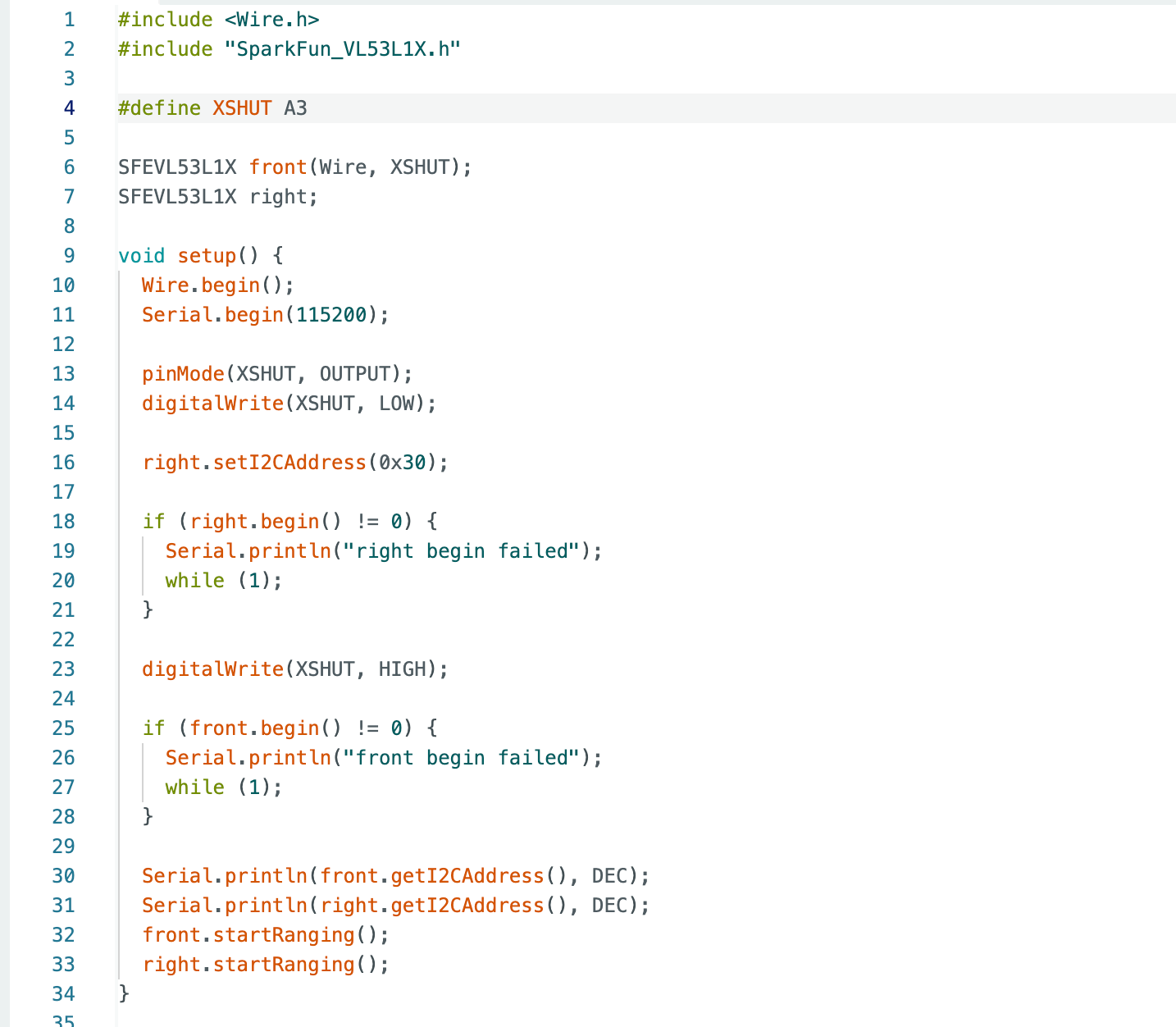
To connect two ToF sensors simultaneously, I changed the address of one sensor to 0x30 during initialization, as shown in the diagram above. The specific procedure is as follows: First, pull the sensor connected to A3 (XSHUT) low to keep it disabled, allowing only the other sensor to operate on the bus and complete initialization; then, I called setI2CAddress(0x30) to change its address from 0x29 to 0x30. Finally, I pulled XSHUT high to enable the second sensor and executed begin() and startRanging() on both sensors. This allows both ToF sensors to operate in parallel on the same I2C bus for normal ranging.
The video above demonstrates that both ToF sensors can successfully perform distance readings.
Task 6: ToF Sensor Speed
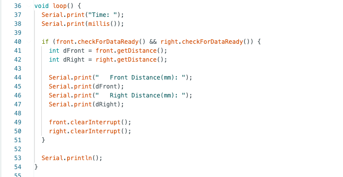
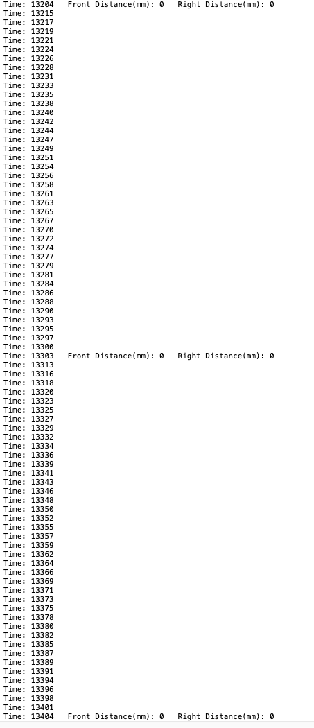
As shown in the code above, to prevent the program from blocking while waiting for the ToF sensors to complete distance measurements, I continuously output the Artemis timestamp using millis() within the loop(). Distance data are read and printed only when both the front and right sensors return checkForDataReady() as true.
From the captured serial output, it can be observed that within the 0.404 s interval from 13204 ms to 13608 ms, “Time:” appeared 159 times. Therefore, the loop execution rate is approximately 393.6 Hz. Meanwhile, “Front Distance(mm)…Right Distance(mm)… ” was output 5 times, corresponding to a new ToF data update rate of approximately 12.38 Hz.
Loop iterations per second = 159 / 0.404 = 393.6 Hz (≈ 394 Hz)
Distance updates per second = 5 / 0.404 = 12.38 Hz (≈ 12.4 Hz)
Therefore, the current bottleneck is not the MCU loop execution, but rather the intrinsic ranging update cycle of the ToF sensors (which requires both sensors to be ready), compounded by the overhead of serial printing and I2C communication. Even though the main loop can execute at a high frequency, distance data can only be produced at the rate at which the sensors generate new measurements.
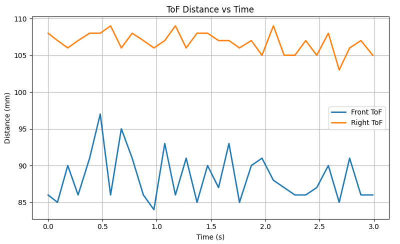
Task 7: Time vs. Distance and Time vs. Angle
In this experiment, the BLE framework developed in Lab 1 was extended to enable
simultaneous acquisition of time-stamped ToF distance data and IMU attitude data within a
fixed recording window. The collected data were then transmitted to the host computer in a
single BLE transfer for subsequent plotting and analysis.
A new Arduino command, READ_IMU_TOF, was implemented. When triggered, the
system continuously records sensor data for approximately 3 seconds. All sensor
measurements share a common time reference defined as
\( t = \text{millis()} - t_{\text{start}} \), ensuring that the ToF and IMU data are aligned on
the same time axis and temporally synchronized.
The figure above shows the ToF distance curve over time. It can be observed that the front distance remains stable within the range of approximately 85–97 mm, while the right-side distance stabilizes within the range of approximately 103–109 mm. The overall trend is relatively smooth, exhibiting only minor fluctuations.
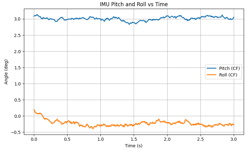
The figure above shows the pitch and roll of the IMU over time. It can be seen that the pitch stabilizes around 3°, while the roll stabilizes around −0.3°. The overall curve is relatively smooth, exhibiting only minor fluctuations.
Additional Task (5000-Level Students)
Task 1: Infrared Transmission Based Sensors Discussion
IR Triangulation Distance Sensors (e.g., Sharp IR)
Principle: An infrared beam is emitted toward the target. The distance is estimated from the position shift of the reflected light on the receiver, based on geometric triangulation.
Advantages: Fast response at close range, simple implementation, and relatively low cost.
Disadvantages: Typically limited measurement range; strongly nonlinear output; sensitive to target color, reflectivity, and surface angle, with large errors for dark or tilted surfaces.
Reflective IR Proximity Sensors (IR LED + Photodiode)
Principle: Measures reflected infrared light intensity, primarily indicating presence or approximate proximity of an object.
Advantages: Very low cost, compact size, easy integration, and fast response.
Disadvantages: Difficult to achieve accurate distance measurement; highly sensitive to ambient light, material, and color; more suitable for near-distance triggering than quantitative ranging.
Time-of-Flight (ToF) Sensors (e.g., VL53L1X)
Principle: Measures the round-trip flight time of emitted light pulses to compute distance.
Advantages: More linear distance output, direct millimeter-level readings, longer range, and well suited for robotic obstacle avoidance and wall-following.
Disadvantages: Update rate limited by ranging cycle parameters (e.g., timing budget); effective range and stability degrade under strong ambient light or low-reflectivity targets.
Task 2: Sensitivity of Sensors
Effect of Color (Reflectivity)
Dark / absorptive materials (black fabric, matte black surfaces): Weak return signal → more prone to jitter, missed detection, or underestimated/unstable readings.
Light / highly reflective materials (white paper, light-colored walls): Strong return signal → generally more stable measurements and longer effective range.
Effect of Texture and Surface Properties
Diffuse surfaces (rough surfaces): Reflections are more scattered but more uniform → often produce more stable readings.
Specular / glossy surfaces (polished metal, mirrors): Specular reflection or multipath effects may occur → occasional distance spikes or jumps.
Transparent / semi-transparent materials (acrylic, glass): Infrared light may transmit through or reflect from the back surface → overestimated or unstable distance readings.
Effect of Incidence Angle (Oblique Targets)
As the angle between the target surface and the sensor optical axis increases, the return signal weakens → higher probability of target loss or reduced measurable range.
Lab 4: Motors and Open Loop Control
Prelab
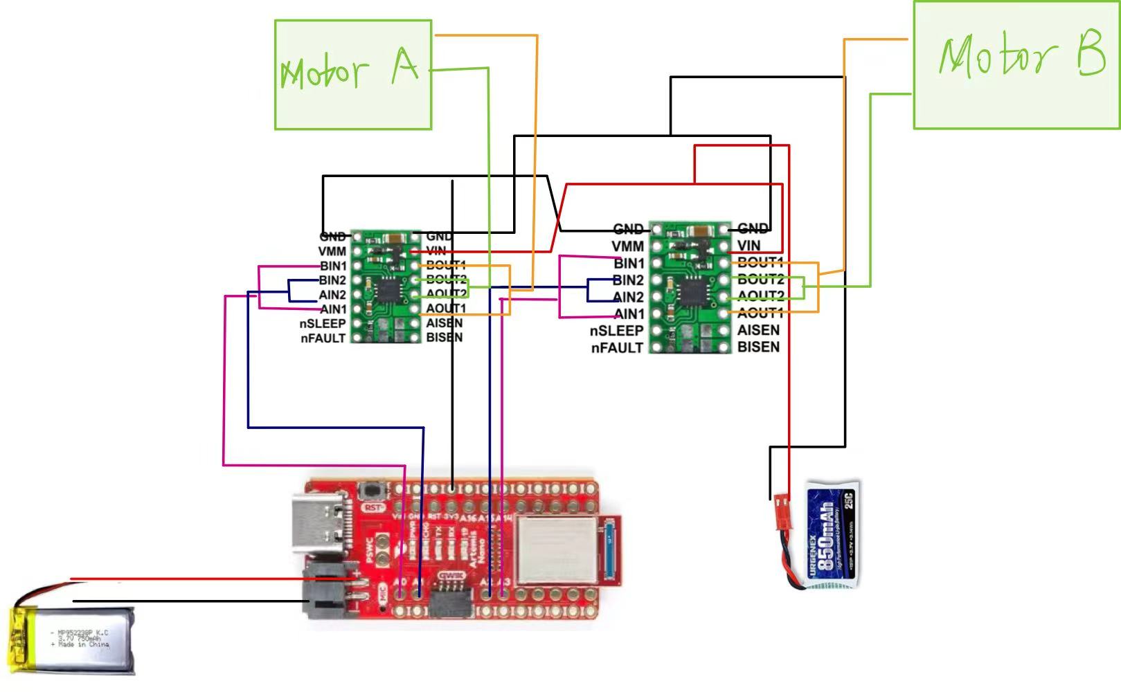
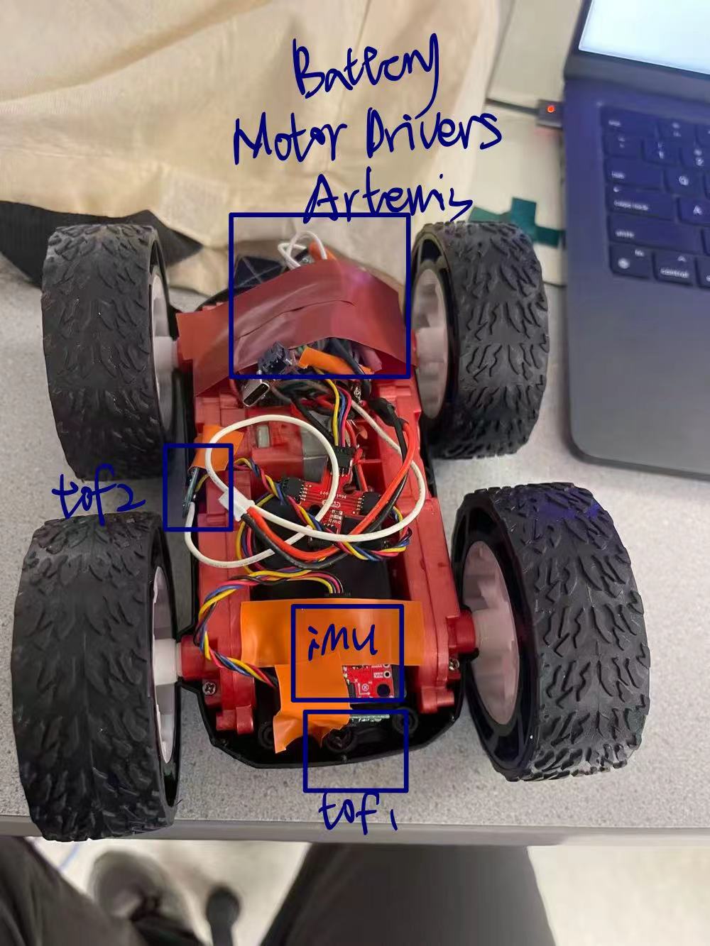
In this experiment, I used two dual motor drivers to control the left and right motors respectively. Following the experiment requirements, I connected the two H-bridge channels of each driver in parallel to increase the current available to the motors. For the left motor, its control inputs AIN1/BIN1 are connected to pin 2 of the Artemis, while AIN2/BIN2 are connected to pin 3. For the right motor, its control inputs AIN1/BIN1 are connected to pin 0, while AIN2/BIN2 are connected to pin 1.
Regarding power connections, the motor driver's VIN/GND terminals are powered by an 850 mAh battery to supply power to the motor, while Artemis is powered by a separate battery.
Task 1: Power Supply Setup
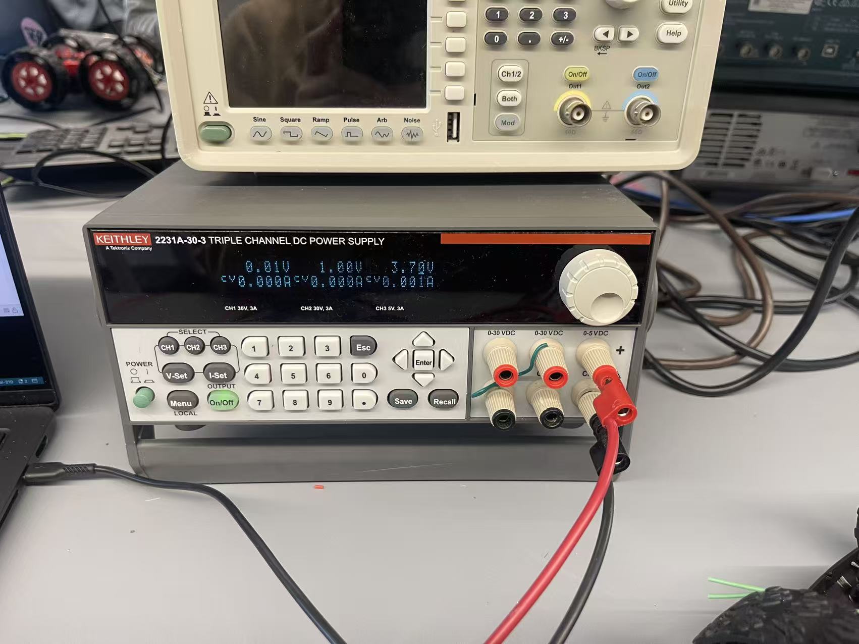
As shown in the figure, we set the power supply voltage to 3.7V, matching the rated voltage of the 850mAh lithium battery to be used later. This ensures that the motor's operating state during debugging aligns with the final battery power supply conditions, preventing test results from deviating from actual operating conditions due to testing at higher or lower voltages.
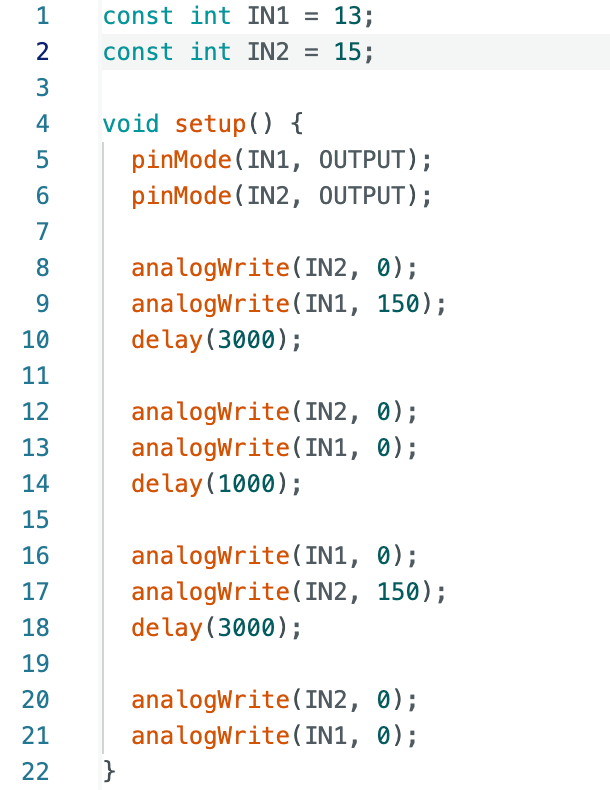
Task 2: PWM Signals
After completing the hardware connections of the motor driver, I used
analogWrite() to generate a PWM signal to regulate the output power of the motor driver.
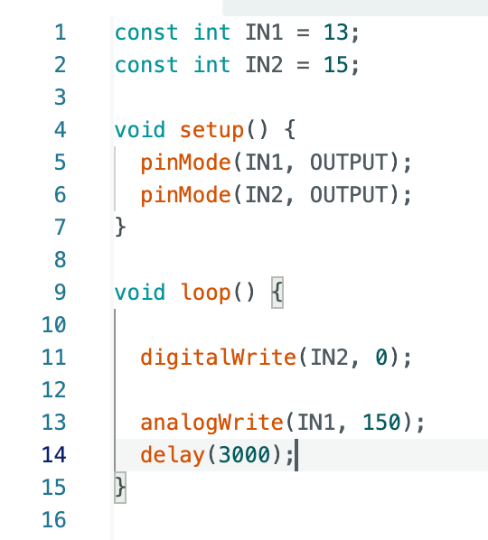
In the program, IN2 was set to a low level to fix the rotation direction, while a PWM signal
was applied to IN1 with a duty cycle value of 150 (within the range of 0–255).
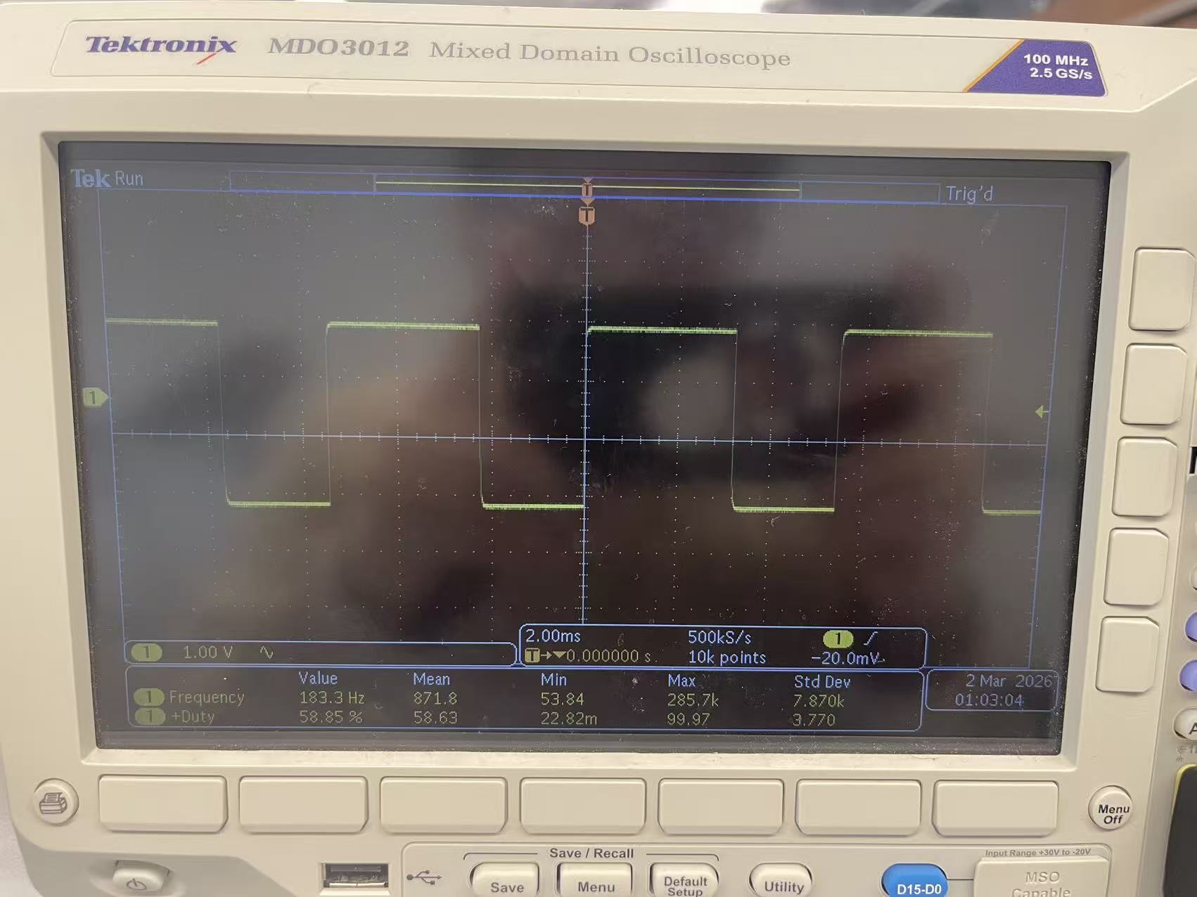
To verify whether the PWM signal is output correctly, I measured the waveform at the driver input using an oscilloscope. The oscilloscope probe was connected to the IN1 pin, with the ground wire connected to the system common ground. The waveform displayed a stable square wave signal with a frequency of approximately 183 Hz and a duty cycle of about 59%, corresponding to the set analogWrite(IN1, 150) value (150/255 ≈ 58.8%). When changing the analogWrite() value, the duty cycle was observed to change accordingly on the oscilloscope.
Task 3: Spinning Wheels with Power Supply
For this section, the external power supply was also set to 3.7 V, and the positive and negative terminals of the circuit were connected to the corresponding terminals of the power supply.
Left Wheel
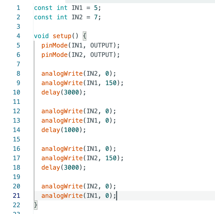
A PWM signal was then applied to the motor driver input. By switching the PWM input configuration to generate forward and reverse rotation, I verified that both motor driver output terminals were able to correctly receive the control signals and drive the motor accordingly.
Right Wheel
The following video demonstrates testing of the right wheel. The operation results align with expectations: it first rotates clockwise and then stops, followed by rotating counterclockwise and stopping.
Task 4: Spinning Wheels with Battery
Left Wheel
After confirming that the motor operates normally when powered by the external power supply, the system was then powered using the provided 850 mAh lithium battery.
The following video demonstrates the wheel's operational state, showing that it rotates as expected.
Right Wheel
The following video shows the right wheel drive in operation.
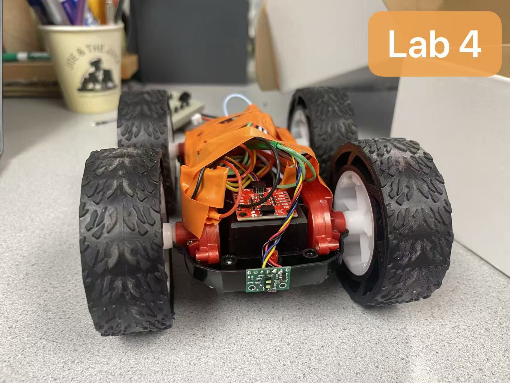
Task 5: Assembled Car
Task 6: Lower Limit PWM
Going Straight
I started with PWM 30. At this point, the motor only emitted a humming sound, insufficient to drive rotation. This indicated the current PWM signal was too weak. I then increased it from 30 to 25, and from 35 to 40. When PWM reached 40, the cart moved slightly but quickly stopped again.
I then tested a PWM value of 45, at which point the car operated normally. Therefore, I determined 45 to be the minimum PWM value for straight-line travel. The following video demonstrates the car's movement.
Turning
To determine the minimum PWM value required for the wheels to overcome friction during turning, I incremented the PWM value from 40 in 10-step increments. The cart only began rotating when the PWM reached 120. The rotation is demonstrated in the following video.
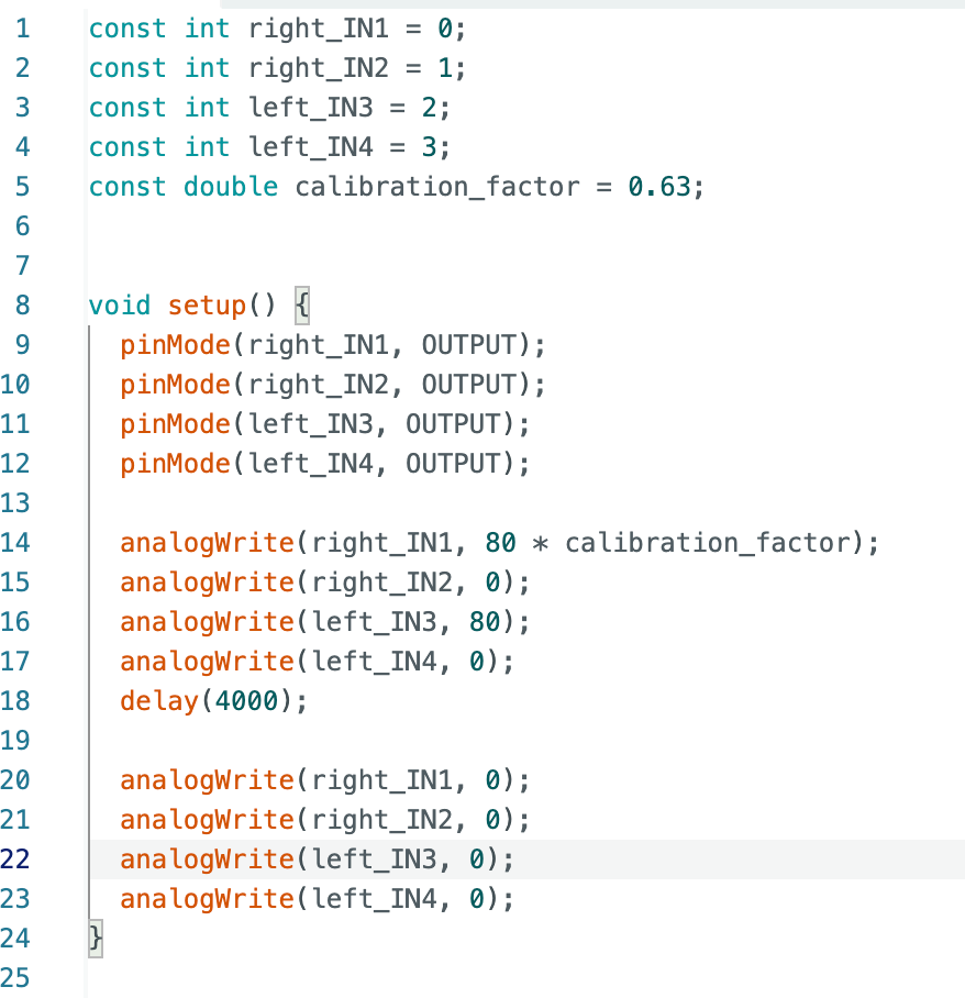
Task 7: Calibration
During previous tests, I observed that the right wheel of the small car rotated faster than the left wheel when receiving identical PWM signals. Therefore, I introduced a calibration factor in the code to scale the PWM of the right motor, thereby balancing the rotational speeds of both wheels. Through iterative adjustments, I determined that 0.63 is the optimal calibration factor when the PWM is set to 80.
The following video demonstrates the calibrated vehicle traveling in a straight line along the tape.
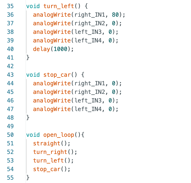
Task 8: Open Loop Control
I predefined a sequence of actions in the program, enabling the robot to execute movements in the order of straight → right turn → left turn → stop without relying on any sensor feedback.
As seen in the video, the robot first moves straight ahead for a distance, then turns right, followed by a turn to the left, and finally comes to a stop.
Additional Task (5000 - Level Students)
Task 1: analogWrite Frequency Discussion
Oscilloscope measurements reveal that the PWM signal generated by analogWrite() on the Artemis board has a frequency of approximately 183 Hz and a duty cycle of about 58.8%, consistent with the program's analogWrite(IN1, 150) setting.
For DC motors, this frequency typically suffices for basic control requirements. However, lower PWM frequencies may cause significant motor current fluctuations and occasionally produce audible motor noise.
Manually configuring the microcontroller's timer to increase the PWM frequency may offer several advantages. For instance, a higher PWM frequency can reduce motor current fluctuations, resulting in smoother output torque. It also helps minimize audible noise, as higher frequencies fall outside the human hearing range. Additionally, higher-frequency PWM enables more stable motor drive, thereby enhancing overall operational performance.
Task 2: Lowest PWM Value Speed Discussion
From the experimental video, it can be observed that starting from the previously measured minimum PWM value of 45, the robot was still able to continue moving forward for a distance when the PWM was reduced to 40. However, after running for a period of time, the robot gradually stopped advancing, with only a faint humming sound emanating from the motor. This indicates that at this PWM value, the torque output by the motor had approached the limit of the system's frictional resistance, rendering it unable to sustain the vehicle's motion.
Therefore, the experiment suggests that PWM = 40 represents the minimum PWM value at which the robot can sustain motion. At lower PWM values, the motor cannot generate sufficient driving force to overcome friction and maintain stable movement.
References
I would like to thank Professor Hebring and teaching assistant Julie for their assistance.
Lab 5: Linear PID control and Linear interpolation
Prelab – BLE Communication
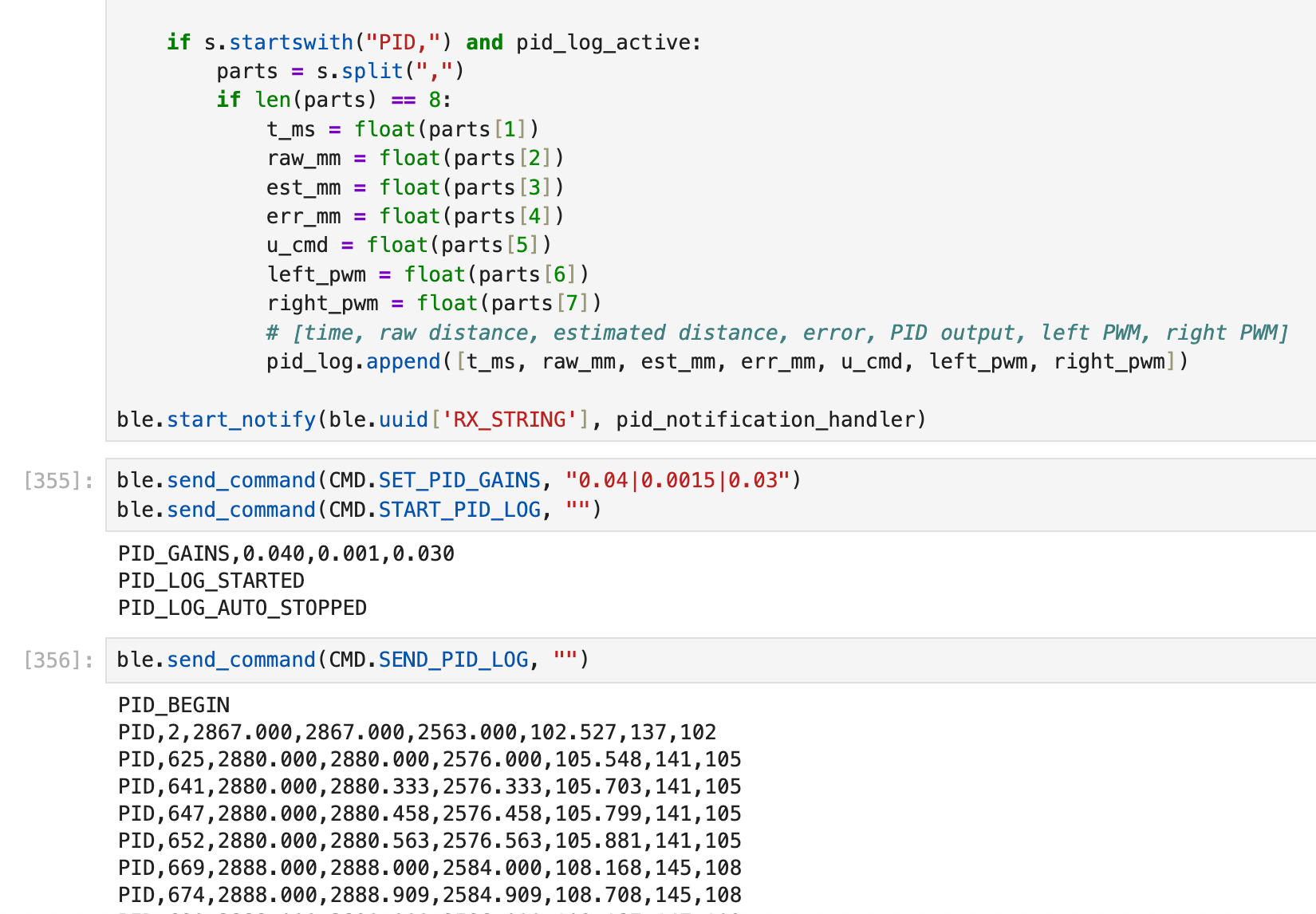
In this lab, Bluetooth Low Energy (BLE) communication was used to control the robot and retrieve experimental data. A Python script running on the computer sends commands to the Artemis board through a BLE characteristic. The Arduino program parses the received command and performs the corresponding operation, such as setting PID gains or starting a PID control experiment.
During a PID test, the robot continuously records data including timestamp, raw ToF distance, extrapolated distance, control error, and motor PWM values. These values are stored in arrays on the Artemis board. After the experiment finishes, the recorded data is transmitted back to the computer through BLE notifications, where Python collects the data and generates plots for analysis of the controller performance.
PID Control and Sampling Discussion
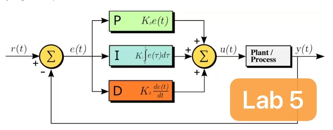
The robot position control uses a standard PID controller.
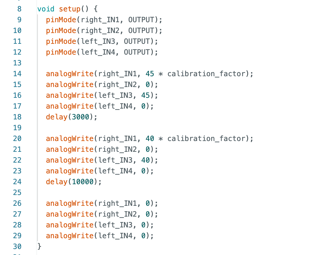
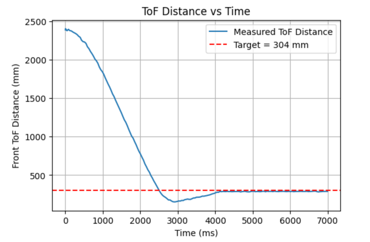
The target distance is set to 304 mm. To compensate for differences in motor performance, a proportional scaling factor is applied to the left and right wheels:
The left wheel rotates more slowly, so additional compensation is applied.
To ensure that the robot approaches the wall quickly when it is far away, the controller is designed so that the robot reaches near-maximum speed at approximately 2000 mm. Since the Arduino PWM limit is 255, the controller’s base PWM is limited to 188, ensuring that the compensated wheel PWM values do not exceed the maximum PWM allowed by the motor driver.
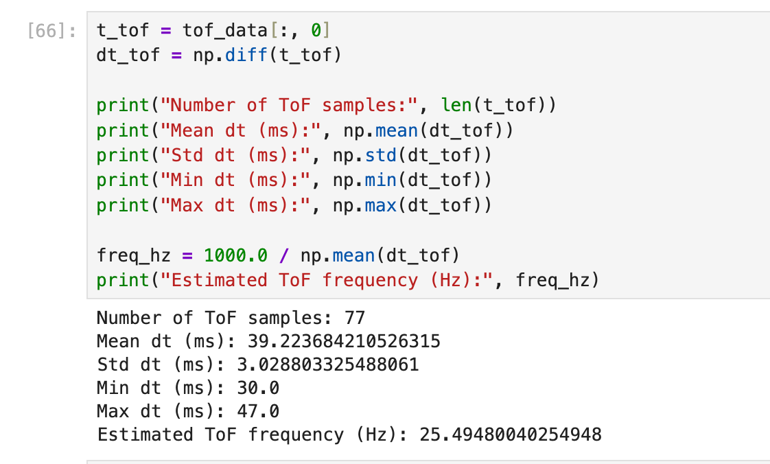
Since the robot’s initial distance from the wall can reach approximately 2000 mm, the long distance mode of the ToF sensor is used to obtain a larger measurement range. Experimental measurements show that the average time interval between two consecutive ToF readings is approximately 39.2 ms, corresponding to a sampling frequency of about 25.5 Hz.
Tuning Process
P control
In the proportional control experiment, I first estimated a theoretical initial value for \(K_p\) based on the target conditions. During the experiment, the robot is expected to move at near maximum speed when it is approximately 2000 mm away from the wall, while the target distance is 304 mm. Therefore, the initial error is approximately
\( e = 2000 - 304 = 1696 \ \text{mm}. \)
The controller output satisfies
\( u = K_p e. \)
Since the goal is for the controller to produce a near-maximum base PWM output of approximately \(u \approx 188\) at this error, we can estimate
\( K_p \approx \frac{188}{1696} \approx 0.11. \)
Therefore, \(K_p = 0.11\) was selected as the theoretical initial value for testing.
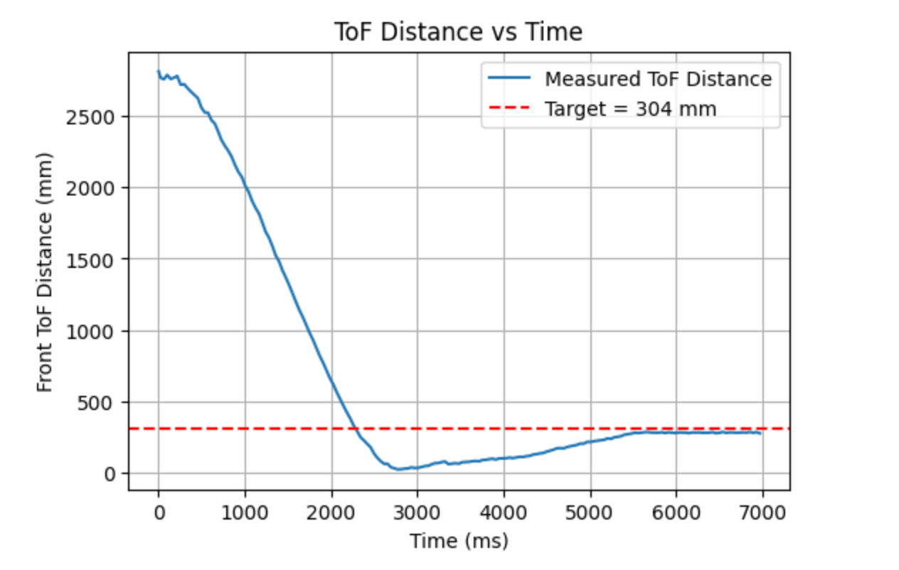
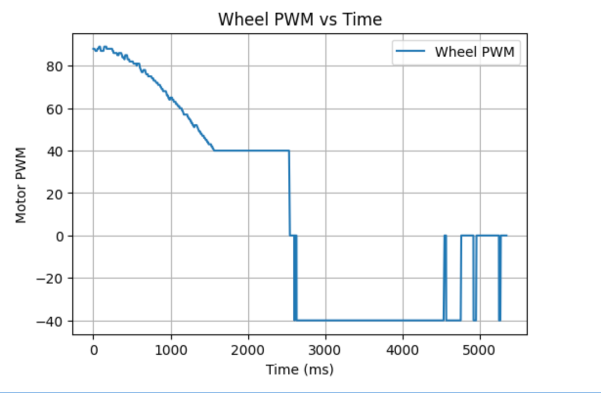
As shown in the figure above, when \(K_p = 0.11\), the robot is able to approach the target position quickly, but the overshoot is very significant and the robot even collides with the wall. To reduce the overshoot and avoid collision, I then gradually decreased the proportional gain and finally selected \(K_p = 0.04\).
However, overshoot was still observed in the experiment. This is likely related to the deadband, the minimum effective PWM, the relatively low ToF sampling frequency, and the inertia of the robot itself. Therefore, a derivative term needs to be introduced to suppress this behavior.
PI control
After introducing the integral term, I gradually increased \(K_i\) to reduce the steady-state error. When \(K_i = 0.0015\), the system reached an acceptable upper limit. Although the integral term could eliminate the error more aggressively, further increasing the integral gain would cause the robot to collide with the wall.
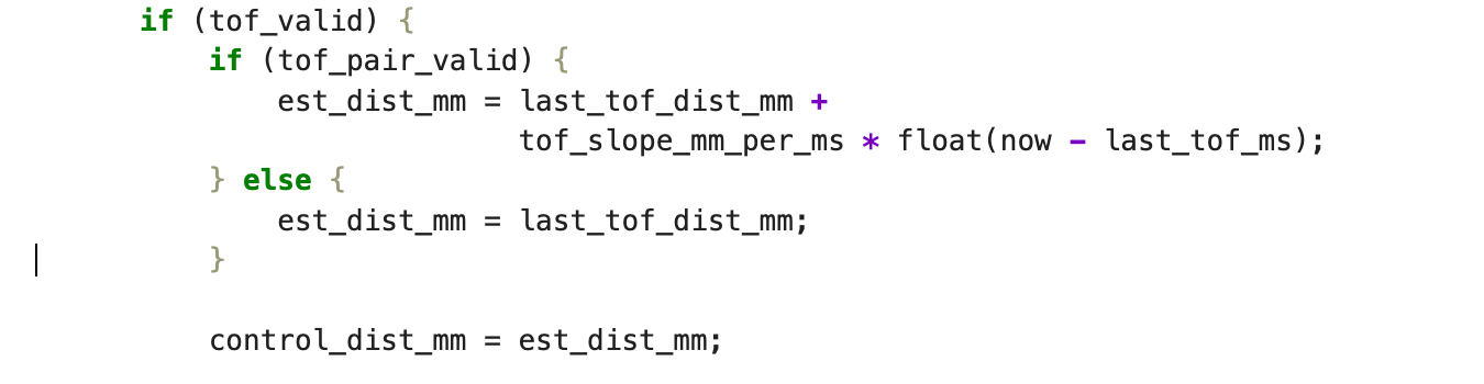
Extrapolation
Since the update frequency of the ToF sensor is about 25.5 Hz, while the PID control loop operates at a higher frequency, waiting for every new ToF measurement would limit the controller performance and cause the distance estimate to change in a step-like manner, which is not suitable for smooth control. Therefore, a linear extrapolation method is introduced.
When no new ToF measurement is available, the two most recent measurements \((d_{k-1}, t_{k-1})\) and \((d_k, t_k)\) are used to estimate the velocity:
\( v = \frac{d_k - d_{k-1}}{t_k - t_{k-1}}. \)
The distance at the current time \(t\) can then be estimated as
\( \hat{d}(t) = d_k + v(t - t_k). \)
This approach generates a continuous distance estimate between two consecutive measurements, allowing the controller to run at a higher frequency while maintaining smoother input to the control system.
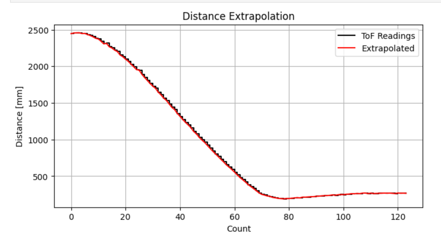
The black curve represents the original ToF measurements, while the red curve represents the extrapolated results. It can be observed that the extrapolated curve closely follows the overall trend of the original measurements while effectively reducing the discontinuities caused by the step-like sampling behavior.
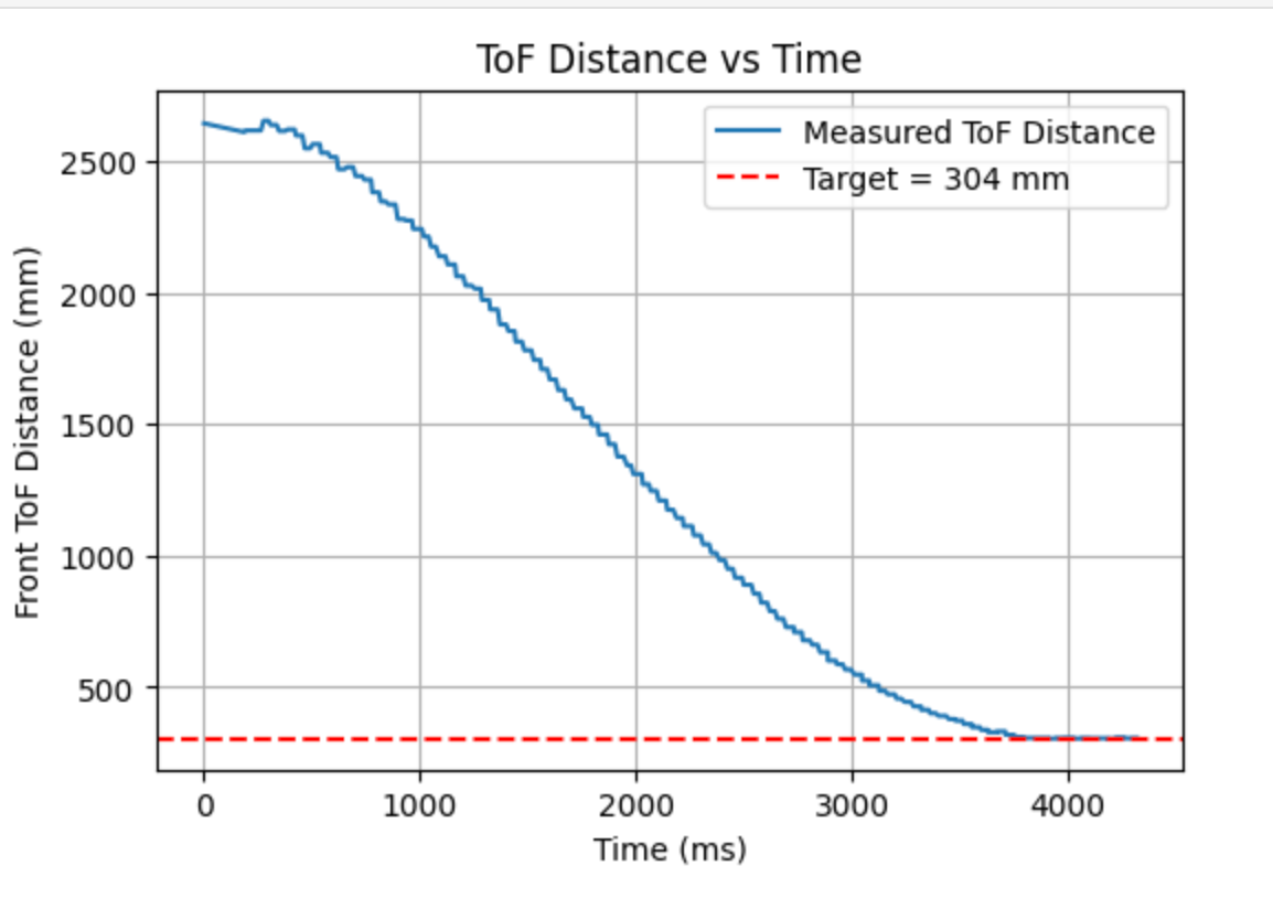
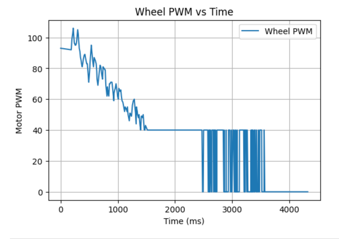
PID control
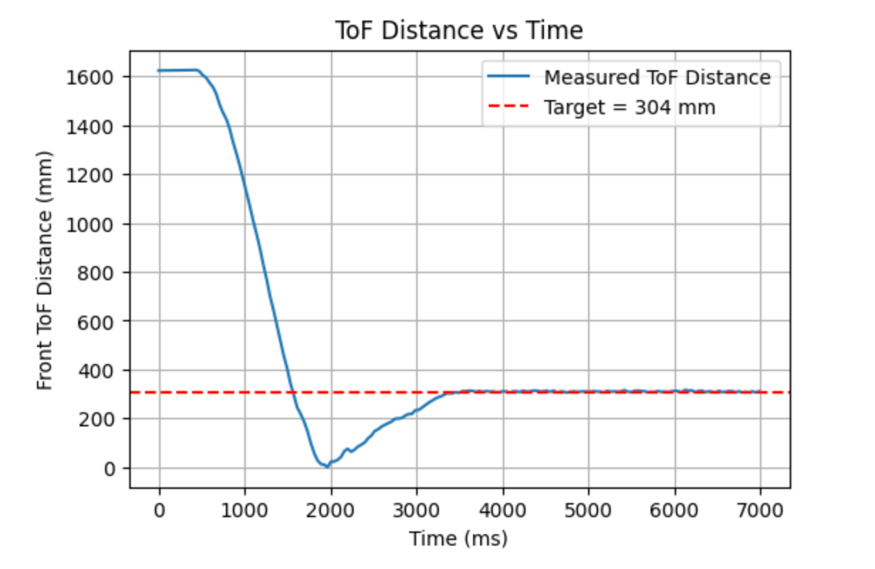
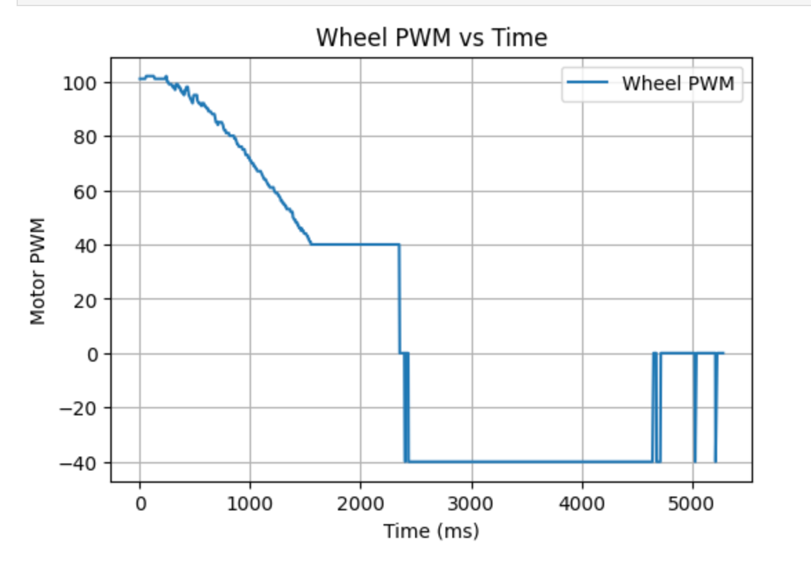
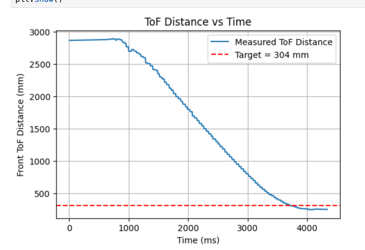
The final selected parameters are \(K_p = 0.04\), \(K_i = 0.0015\), and \(K_d = 0.03\). From the figures, it can be observed that the ToF distance curve decreases smoothly overall and gradually converges as the robot approaches the target position. Correspondingly, the motor PWM also gradually decreases as the control error becomes smaller.
Testing result
The following three videos demonstrate the robot automatically stopping at the target distance.
The following video demonstrates the robot's ability to resist external disturbances.
Additional Task (5000-Level Students)
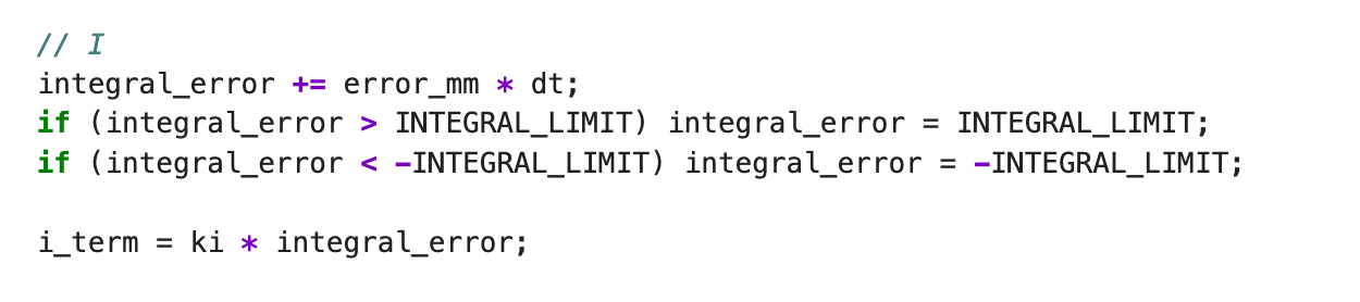
I adopted the simplest integral limiting method by setting upper and lower bounds on the integral error integral_error to prevent unlimited accumulation. The code uses
The figure on the right shows the results after removing the wind-up protection. The robot exhibits larger overshoot as it approaches the target position. After applying the integral limit, the system converges more smoothly and stabilizes more easily near the target distance.
References
This experiment referenced the course website created by Katherine Hsu.
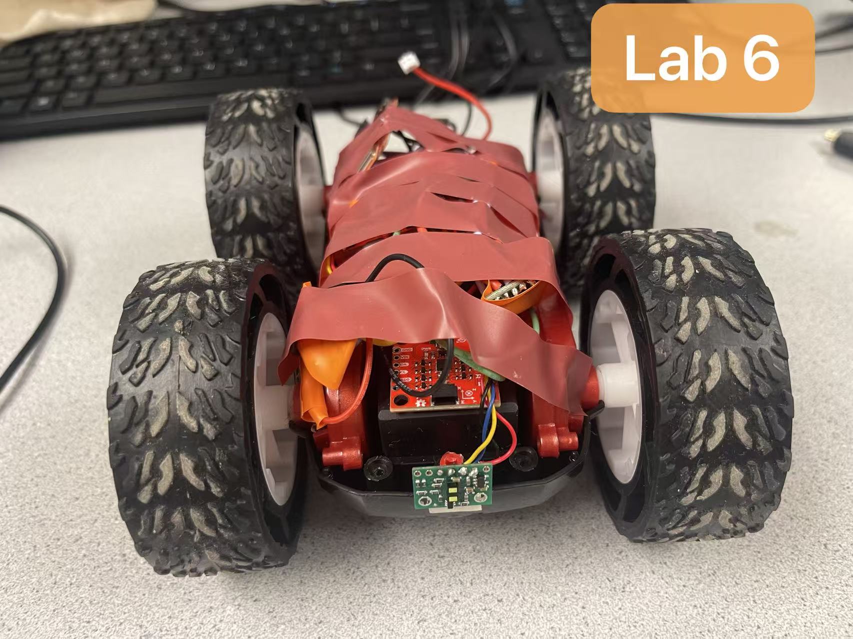
Lab 6: Orientation Control
Prelab
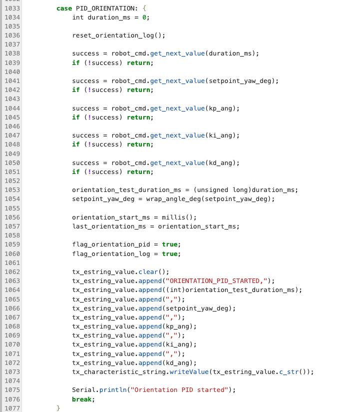
For the orientation control experiment in this lab, I implemented a command called PID_ORIENTATION. This command is used to set the control duration, define the target angle (setpoint), configure the controller parameters (Kp, Ki, Kd), and start the orientation control along with data logging.
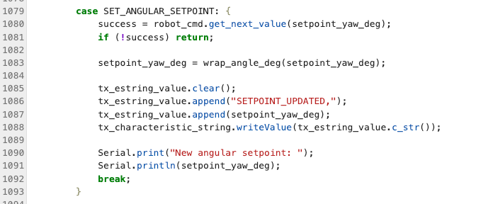
To support dynamic control, I also implemented a separate SET_ANGULAR_SETPOINT command to update the target angle during runtime.
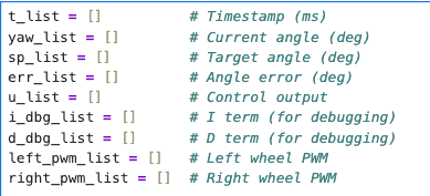
During the orientation control process, the robot records one data sample at each control cycle and stores it in an array, including
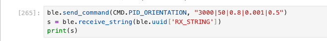
You can send commands to the robot via BLE from your computer.
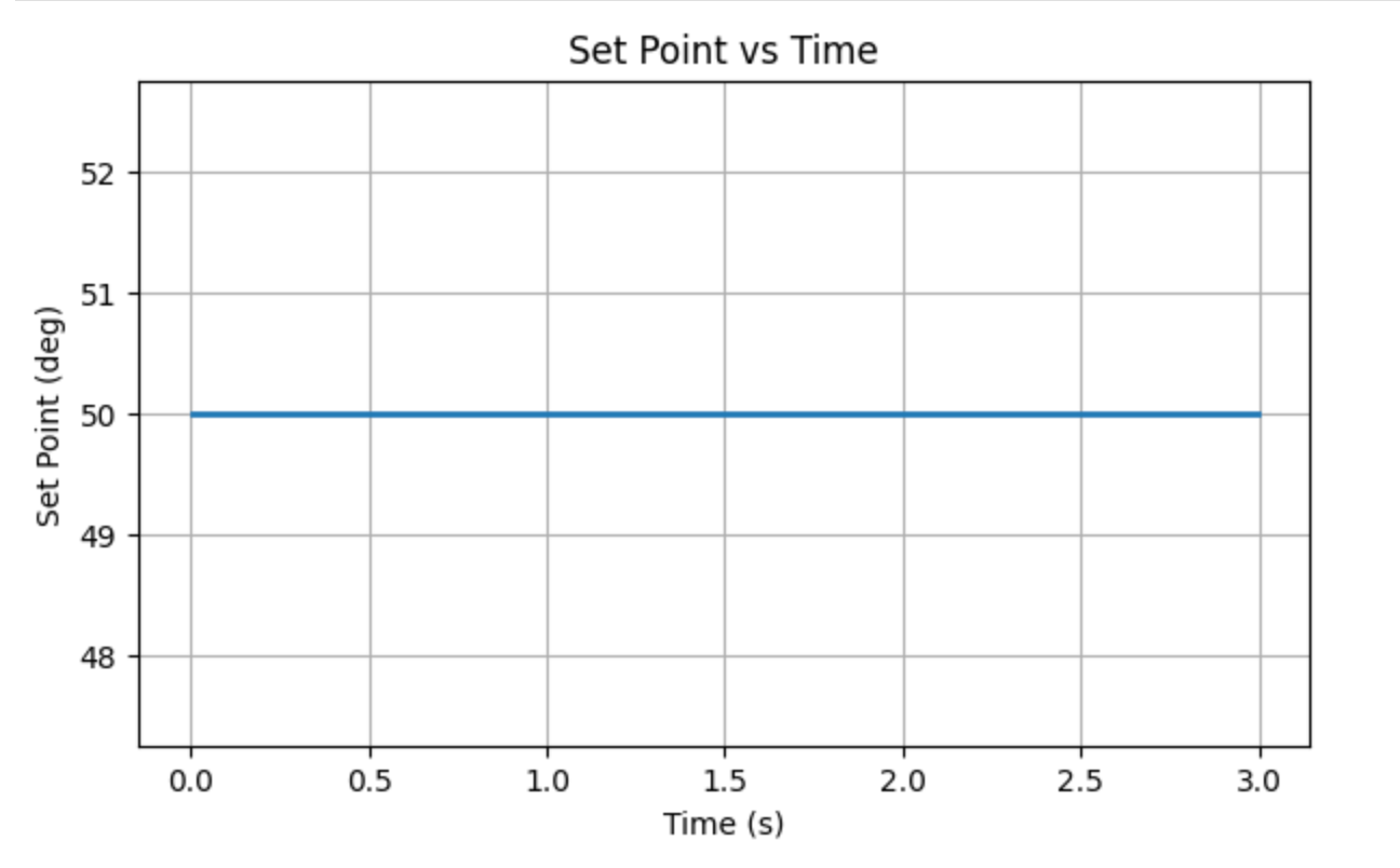
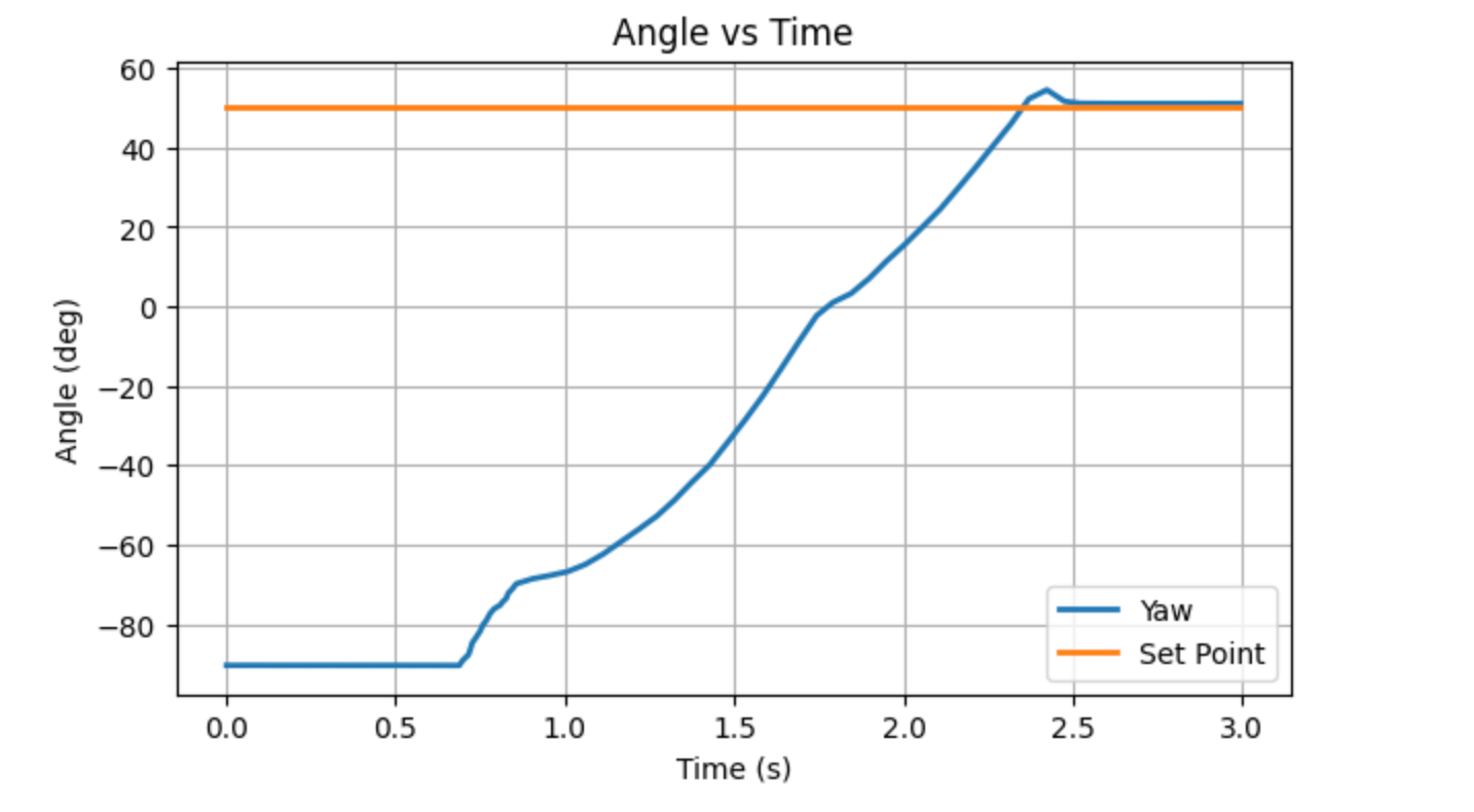
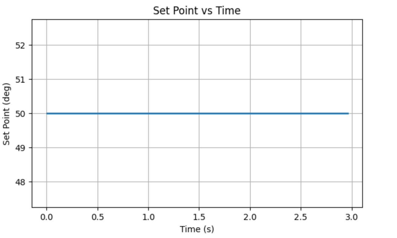
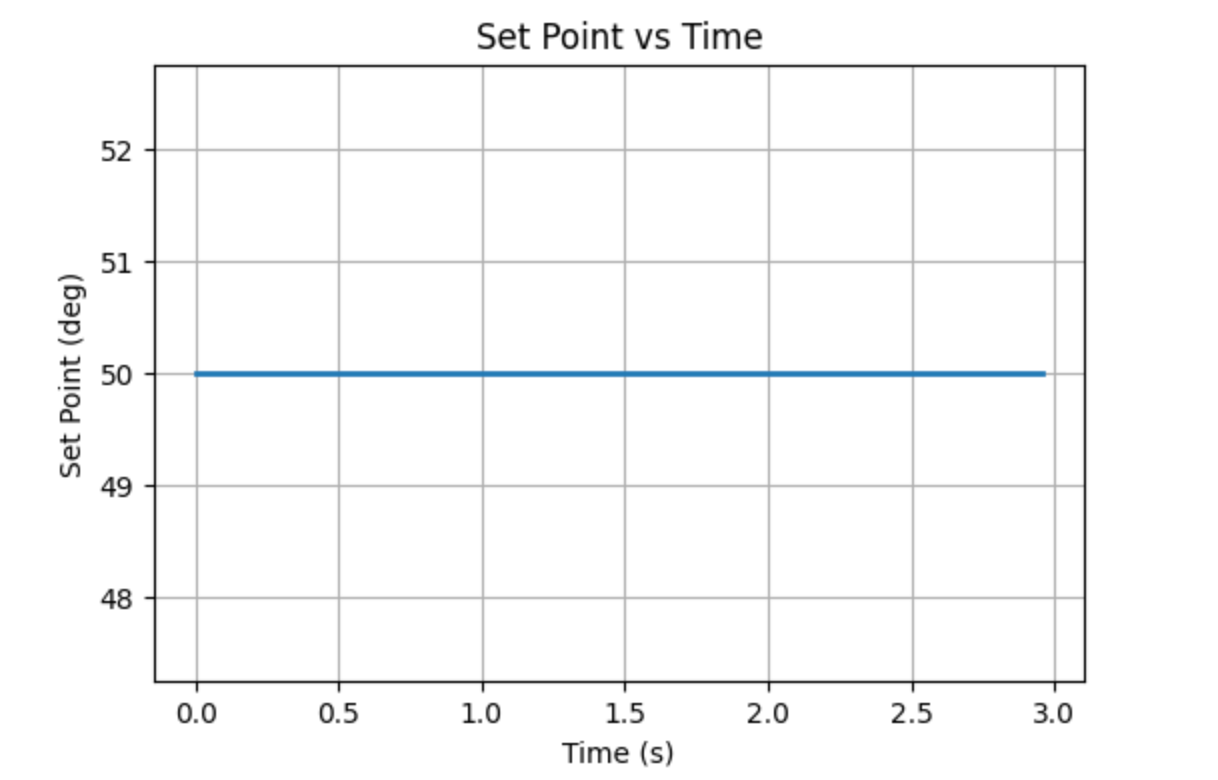
This command specifies a control duration of 3 seconds, a target angle of 50°, and controller parameters of \(K_p = 0.8\), \(K_i = 0.001\), and \(K_d = 0.5\).
Part 1: Orientation Control
To realize in-place orientation control, I apply differential drive by letting left and right wheels rotate in opposite directions.
This corresponds to differential drive as follows:
Turn right: left wheel forward, right wheel backward
Turn left: left wheel backward, right wheel forward
Part 2: PID Input Signal
For orientation control, it is necessary to estimate the robot's current yaw angle. The most straightforward approach is to integrate the gyroscope angular velocity. However, this method suffers from drift over time. Even when the robot is stationary, gyroscope bias leads to accumulated error in the estimated angle.
To mitigate this drift, the IMU's built-in DMP is used to directly output orientation data. The DMP can directly output orientation in the form of quaternions, which significantly reduces yaw drift and makes it more suitable as the input signal for the PID controller.
In implementation, the DMP is first enabled by uncommenting the following line in the library file ICM_20948_C.h:
#define ICM_20948_USE_DMP
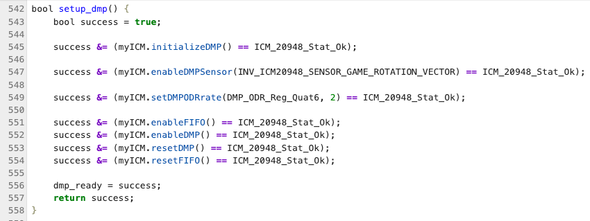
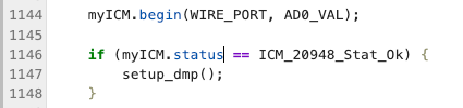
Then, following Example7_DMP_Quat6_EulerAngles.ino to initialize the DMP.
Call this after initializing the IMU in setup()
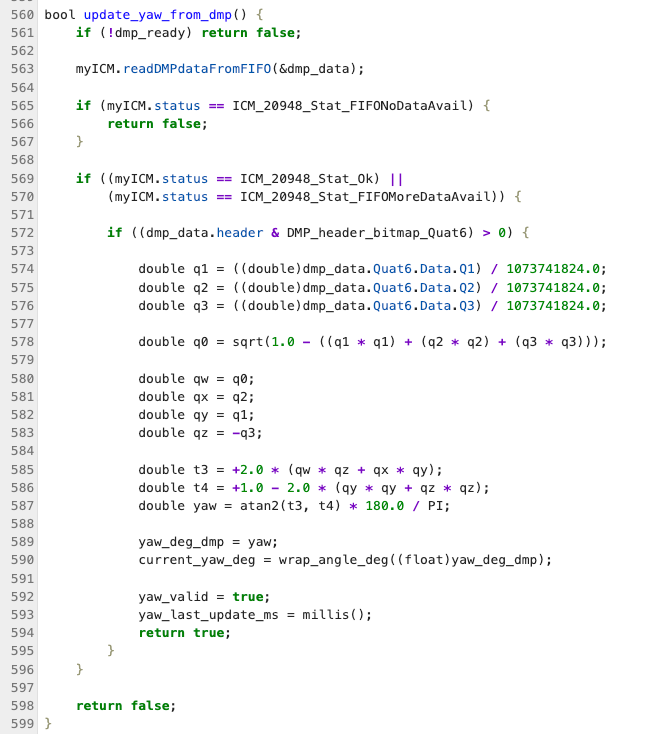
In the main loop, DMP data is read from the FIFO and the yaw angle is calculated
During the control loop, this function is continuously called, and current_yaw_deg is used as the input to the PID controller.
In terms of sensor limitations, the IMU gyroscope has a maximum range of ±2000 deg/s, which is sufficient for the in-place rotation required in this experiment and does not require additional configuration.
In addition, when the PWM is below approximately 125, the motors do not rotate. Therefore, a minimum PWM threshold is applied.
Part 3: Derivative Term
In this experiment, the orientation control error is defined as the difference between the current yaw angle and the target yaw angle. Since this error is obtained from discretely sampled angle measurements, it is reasonable to compute its derivative.
The derivative term reflects the rate of change of the error. When the robot approaches the target angle rapidly, the derivative term provides a damping effect that counteracts the motion, thereby reducing overshoot and improving convergence speed.
When the setpoint changes during operation, the error experiences an instantaneous jump, which leads to a spike in the derivative term (known as derivative kick), causing a sudden change in the control output.
Since the derivative term is sensitive to noise, a low-pass filter is required in practical implementation to smooth the output. After applying the filter in this experiment, the control becomes more stable, making it a necessary improvement.
Part 4: Programming Implementation
This experiment adopts a non-blocking control structure to implement orientation PID control. When the PID_ORIENTATION command is received, only the control parameters are updated and a control flag is set, while the main loop continues to perform orientation updates and control computations.
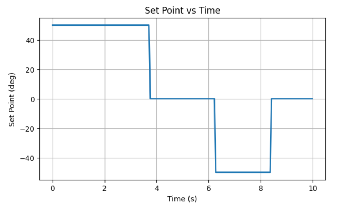
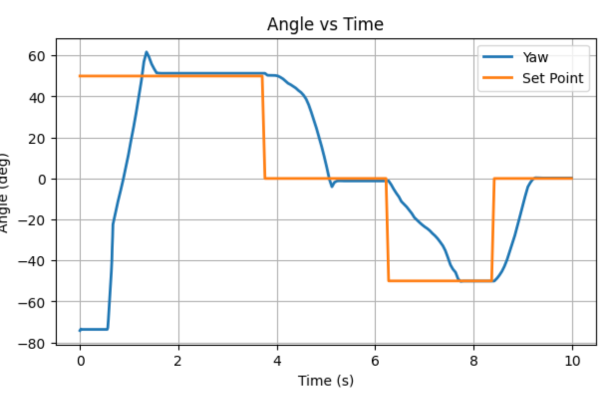
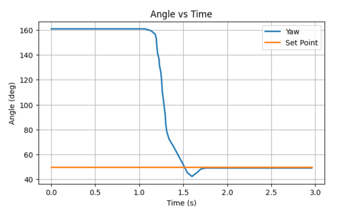
To verify this functionality, I set the target angle sequentially to \(+50^\circ \rightarrow 0^\circ \rightarrow -50^\circ \rightarrow 0^\circ\) during a single run. The results are shown below:
It can be observed that the yaw angle follows the changing setpoint and gradually converges to the target angle.
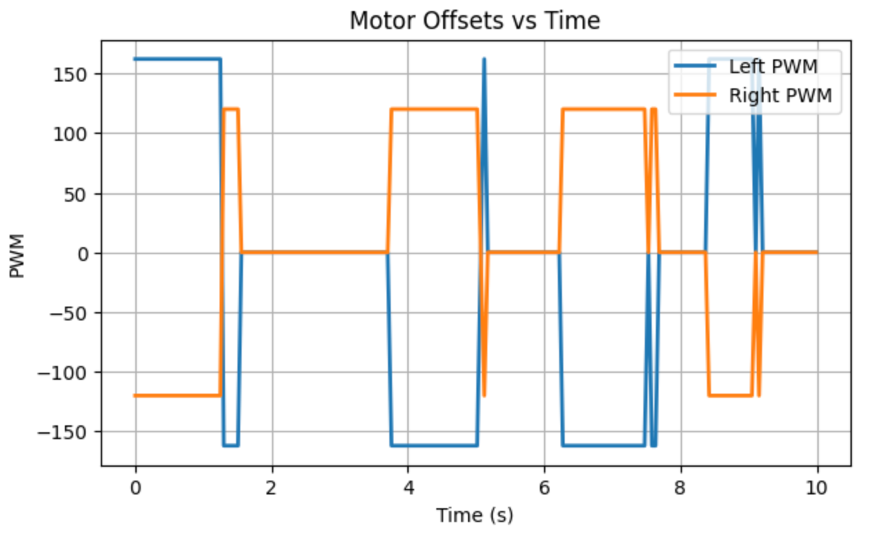
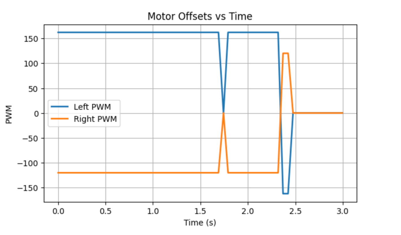
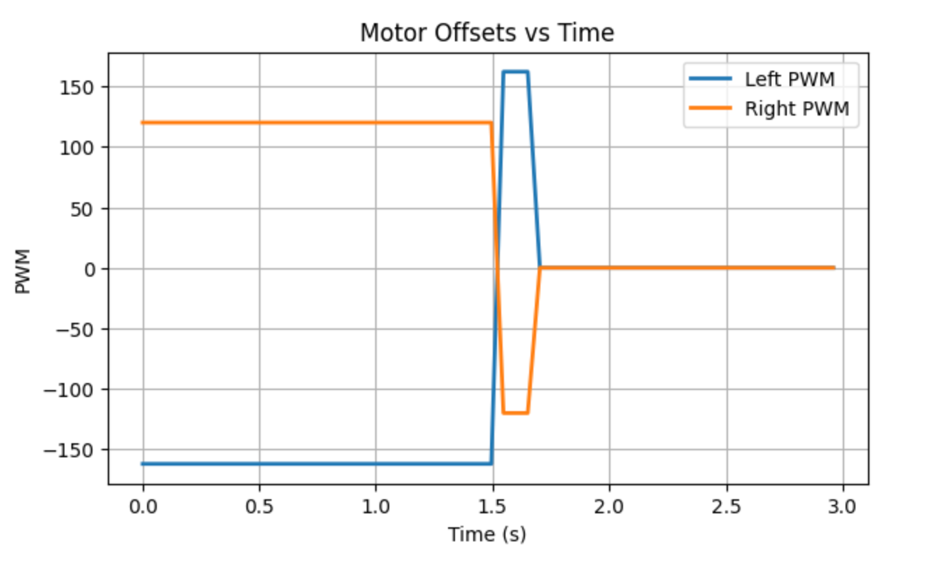
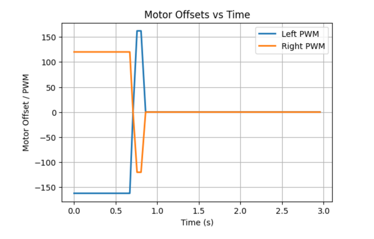
The corresponding PWM curves show that the left and right wheels alternately reverse direction, enabling orientation adjustment.
The following video demonstrates the robot’s actual turning behavior.
In future navigation or advanced applications, real-time setpoint updates are essential, as the robot needs to continuously adjust its target heading during operation rather than restarting the controller each time.
Regarding whether orientation can still be controlled while the robot is moving forward or backward, this functionality was not explicitly implemented in this experiment. However, the current program has already modularized the orientation control logic. By combining linear velocity control and angular velocity control into the left and right wheel PWM signals, heading correction can be incorporated during motion.
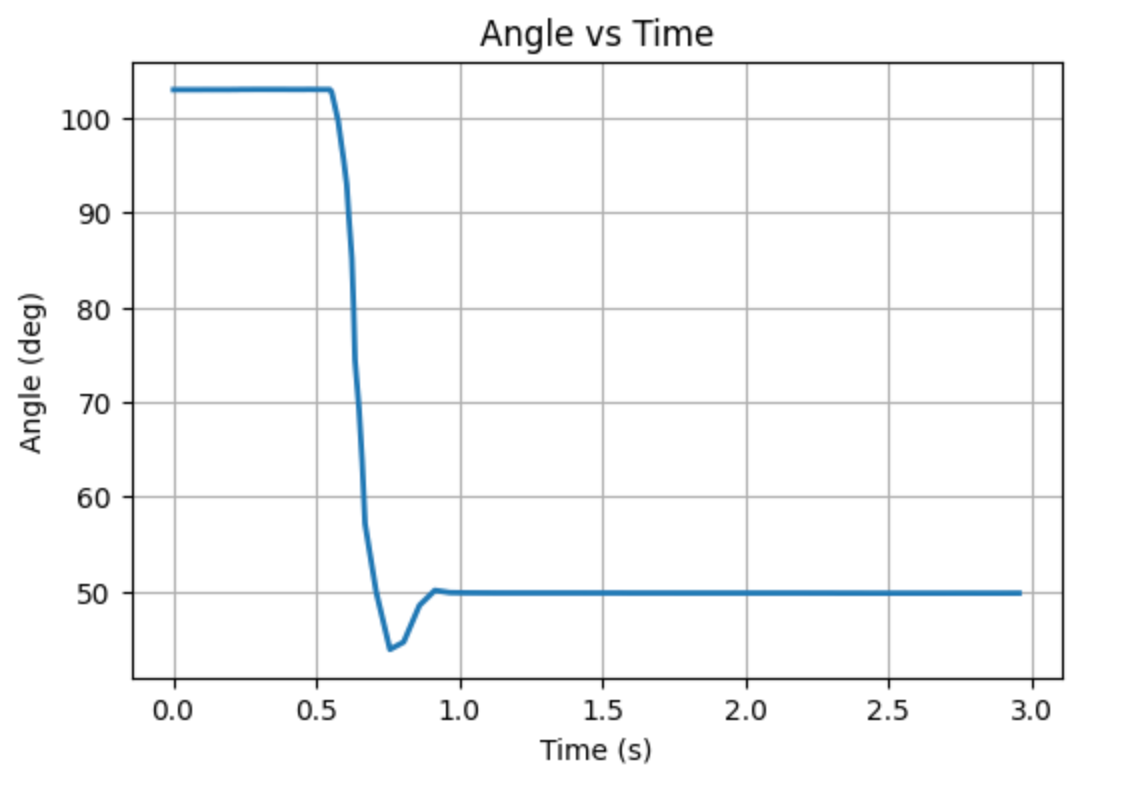
Part 5: Results
The final tuned gains are \(K_p = 0.8\), \(K_i = 0.001\), and \(K_d = 0.5\). To validate the reliability of the results, the experiment was repeated three times.
Trial 1
Trial 2
Trial 3
Disturbance Rejection Test
The following video demonstrates the disturbance rejection test. It can be observed that when I manually change the robot’s orientation using my foot, it is able to automatically correct itself and return to the target heading.
Additional Task (5000 - Level Students)
For the integral term, wind-up protection is introduced by limiting it within the range \([-100, 100]\).
This is necessary because when the error is large or the motor output is already saturated, the integral term may continue to accumulate, leading to excessive control output and causing significant overshoot and oscillations. By constraining the integral term, over-accumulation is prevented, resulting in more stable behavior under different surface conditions and faster convergence.
References
This project referenced the course websites of Katherine Hsu and Evan Leong.
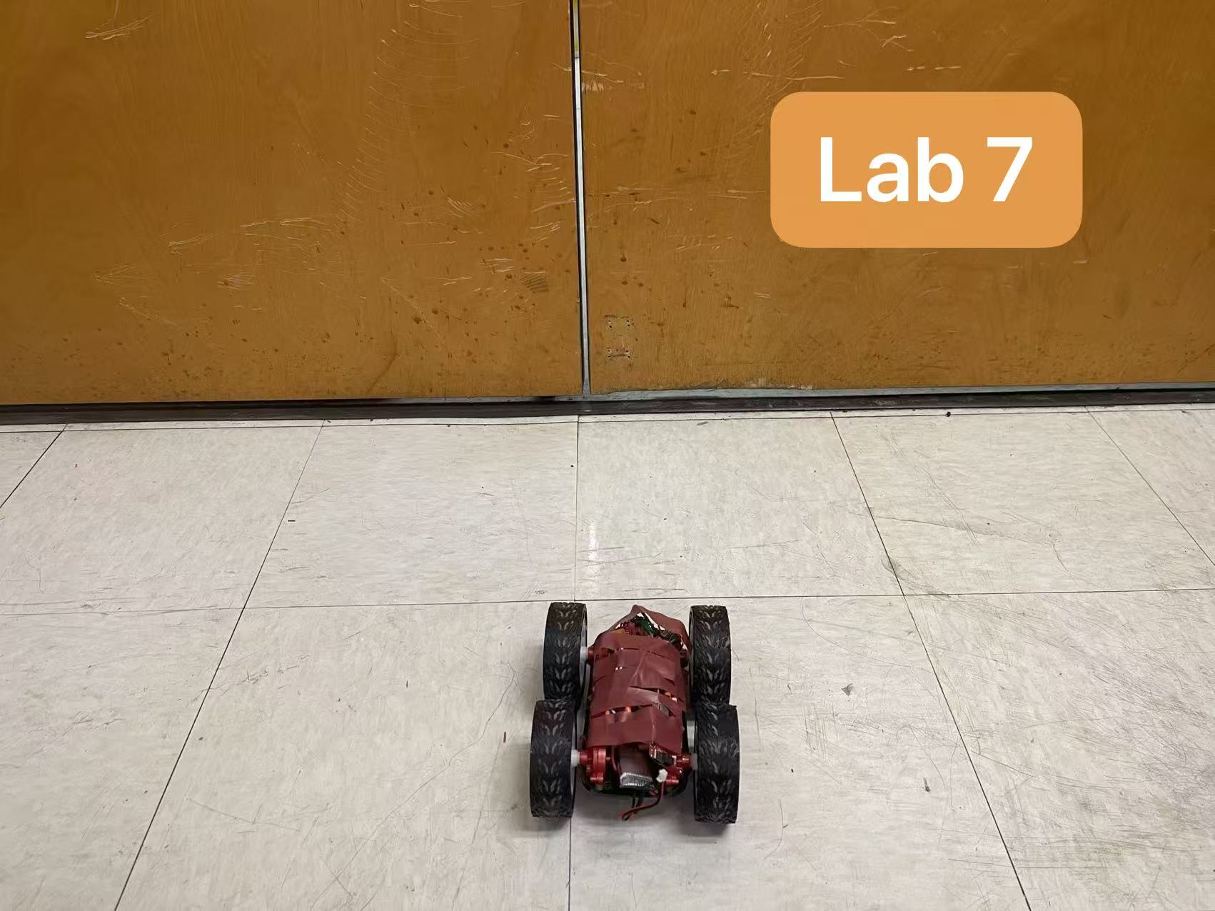
Lab 7: Kalman Filter
Prelab
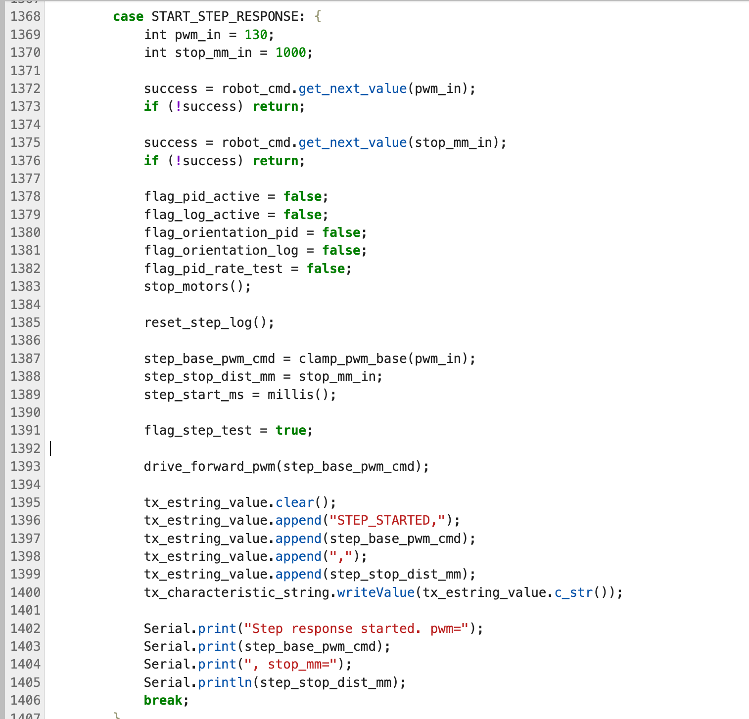
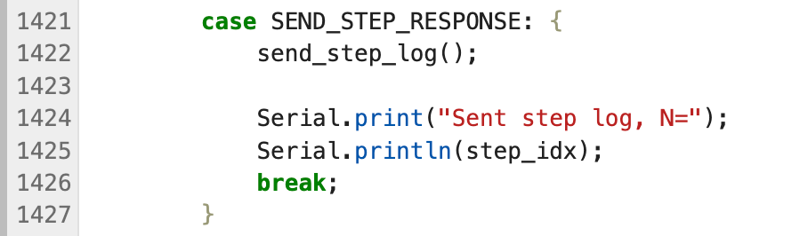
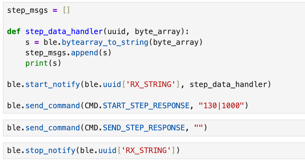
First, I added commands related to step response for drag and momentum estimation in Part 1. The START_STEP_RESPONSE command is used to initiate a linear test with a fixed PWM, while the SEND_STEP_RESPONSE command is used to send the recorded timestamps, ToF, and PWM data back to the computer.
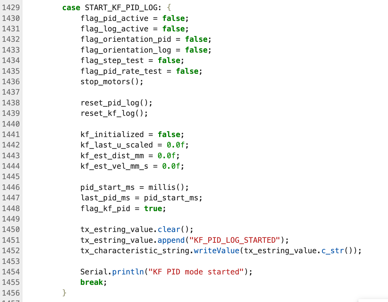
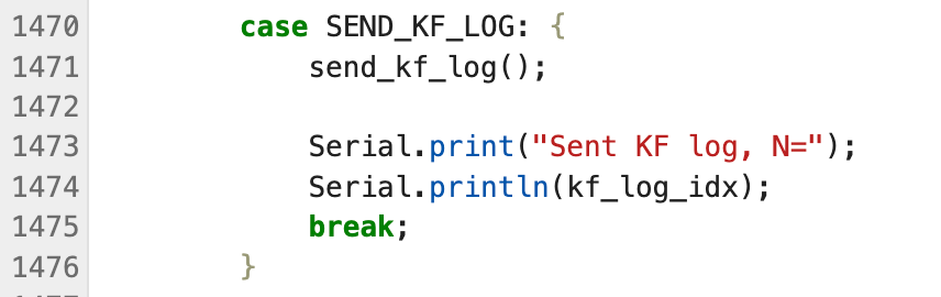
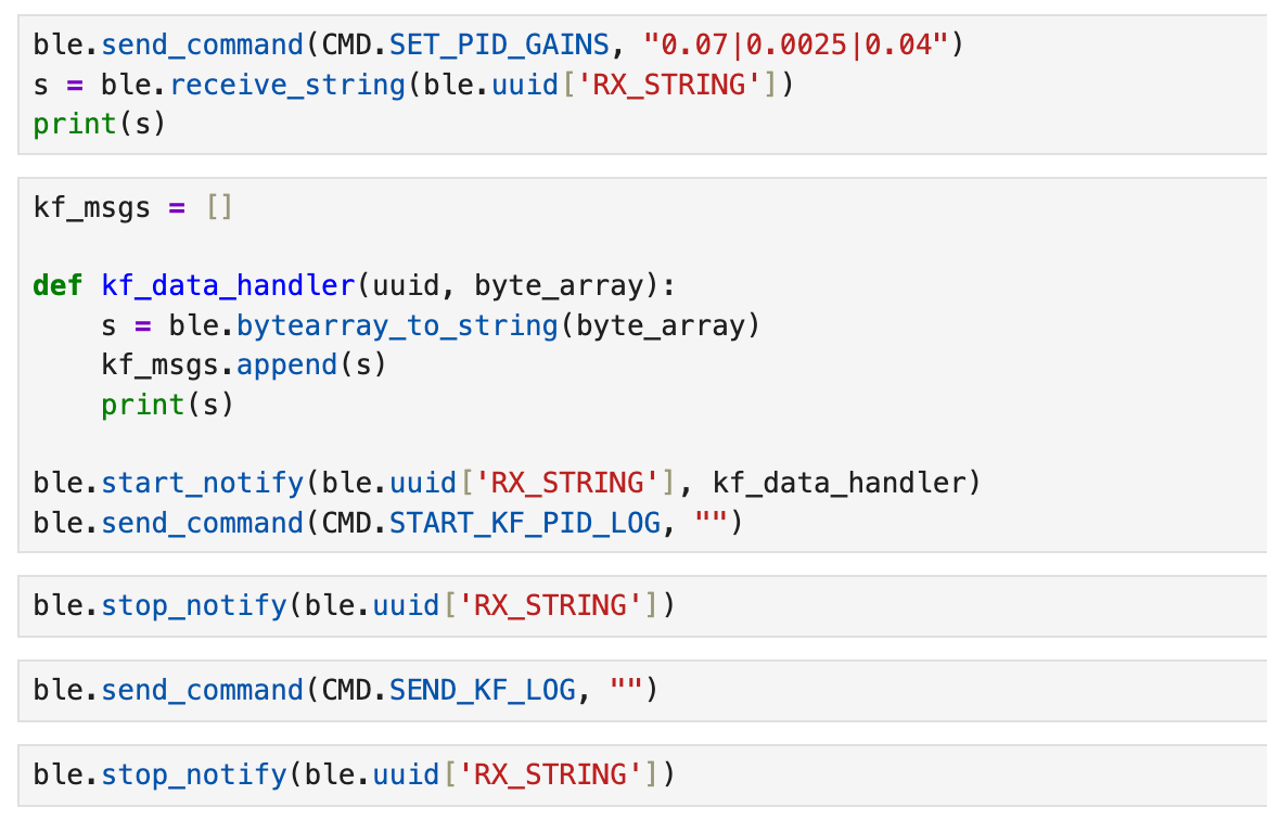
To support the Kalman Filter experiment on the robot side in Part 4, I have added new commands related to KF-PID logging. The START_KF_PID_LOG command is used to initiate Kalman Filter-based distance estimation and PID control, while the SEND_KF_LOG command is used to transmit recorded raw ToF data, KF-estimated distance, estimated velocity, and scaled control inputs.
On the computer, I can launch step response or KF-PID experiments directly through Notebook and receive log strings asynchronously, which I can then parse into arrays for plotting and saving data.
Part 1: Estimate Drag and Momentum
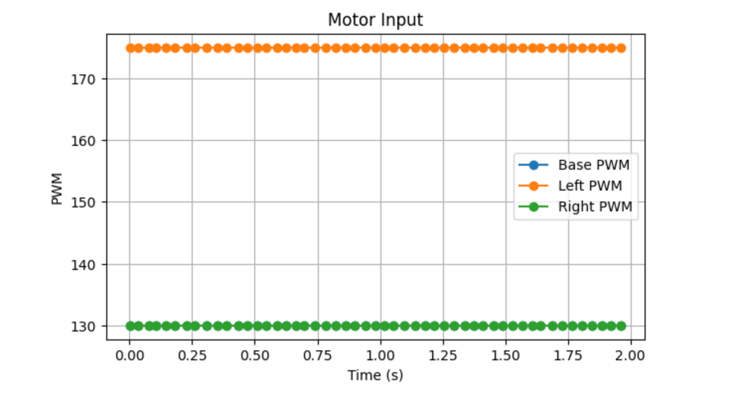
In this experiment, I had the robot move in a straight line toward the wall at a fixed motor input, while simultaneously recording the ToF distance, timestamps, and motor input data. Since the output of the left and right wheels was not exactly the same, I set the base PWM to 130 and applied compensation to the left wheel. To prevent the robot from colliding with the wall, it automatically stopped when the ToF reading approached 1000 mm.
The figure below shows the motor input curve. As can be seen, the input remains constant throughout the entire step response, which satisfies the basic conditions for first-order system response analysis.
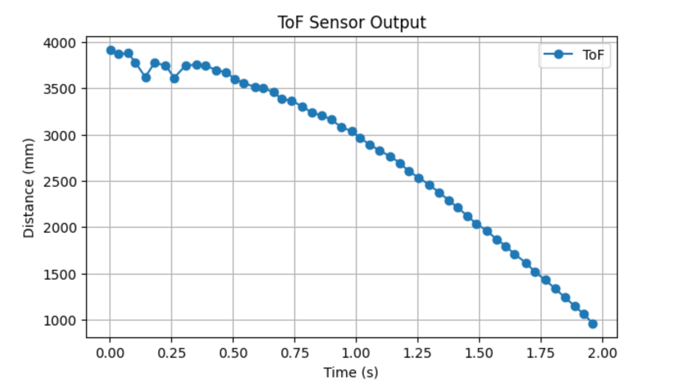
Next is the ToF distance curve, which shows the robot gradually approaching the wall from a distance of approximately 3,900 mm and stopping at around 1,000 mm.
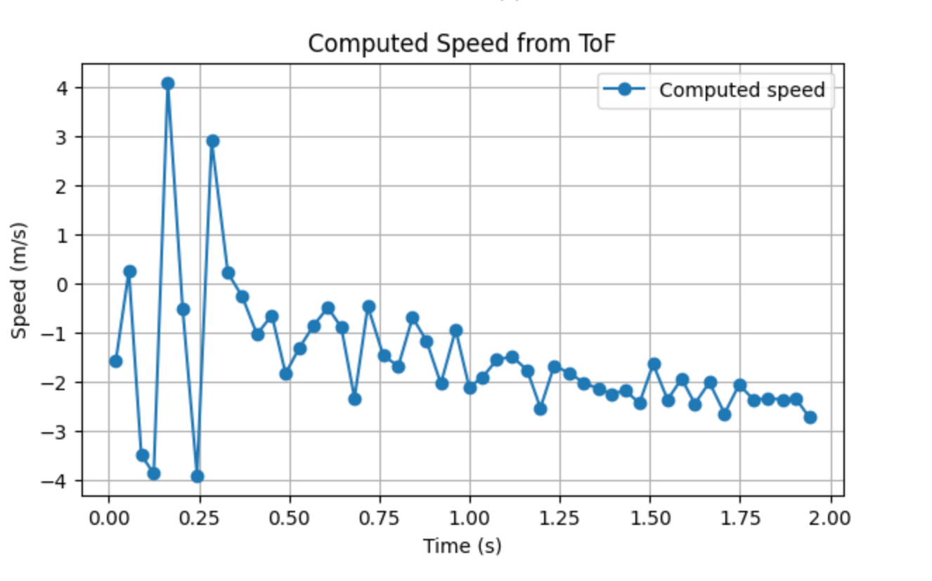
To estimate the system speed from the step response, I differentiated the ToF data to obtain a velocity curve.
Based on this data, the steady-state speed was ultimately determined to be vss ≈ 2.281 m/s, and the 90% steady-state speed is 0.9vss ≈ 2.053 m/s, and the corresponding 90% rise time is t0.9 ≈ 1.355 s, and the velocity at the time corresponding to the rise time is approximately v(t0.9) ≈ 2.086 m/s.
Let the normalized input be \( u = 1 \).
According to the steady-state relationship
\[
d = \frac{u}{\dot{x}_{ss}}
\]
we obtain
\[
d = \frac{1}{2280.8} \approx 4.38 \times 10^{-4}
\]
Next, the 90% rise time is used to estimate the momentum term,
\[
m = \frac{-d\,t_{0.9}}{\ln(0.1)}
\]
Substituting \( d \approx 4.3845 \times 10^{-4} \) and \( t_{0.9} \approx 1.3546 \,\text{s} \) gives
\[
m \approx 2.58 \times 10^{-4}
\]
Therefore, in the subsequent Kalman Filter initialization, the system parameters I used are
\[
d \approx 4.38 \times 10^{-4}, \qquad
m \approx 2.58 \times 10^{-4}
\]
Part 2: Initialize KF
After obtaining the estimated drag term d and momentum term m from Part 1, I first constructed the system state-space model in Python. The system state is defined as distance and velocity, so the state vector is written as
\[
\mathbf{x} =
\begin{bmatrix}
x \\
\dot{x}
\end{bmatrix}
\]
Part 3: Implement and Test your Kalman Filter in Jupyter
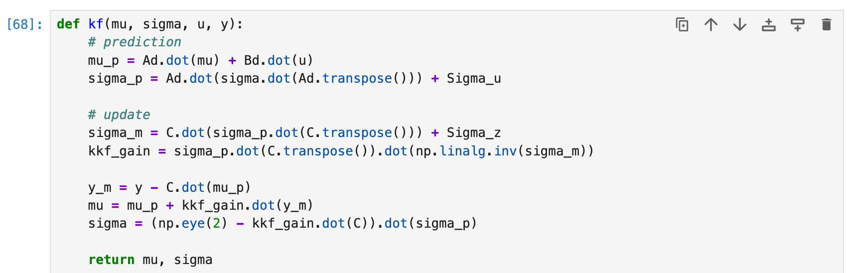
I first implemented the Kalman Filter function based on the prediction-update structure described in the lecture.
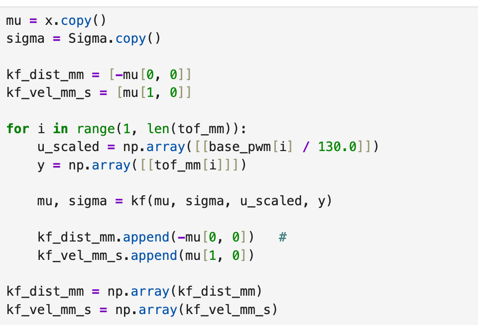
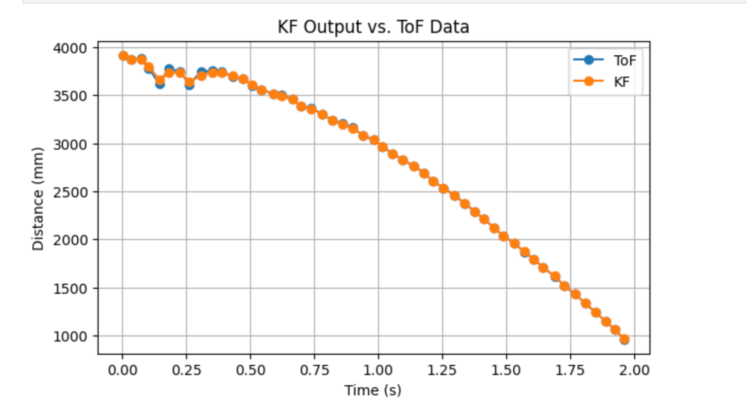
Then, I used the initialized \( \mathbf{x} \) and \( \Sigma \) from Part 2 as the initial values of the filter and ran the Kalman Filter point by point on the step response data. Since the step input in this experiment was set to 130, the motor input was scaled as \( u/130 \) at each step. Because the position in the state is defined as negative distance, it was converted back to a positive distance when saving the results so that it could be directly compared with the raw ToF data.
As can be seen in the figure, the KF output closely follows the overall trend of the ToF distance curve and largely coincides with the raw measurements for most of the time.
Part 4: Implement the Kalman Filter on the Robot
In this section, I integrated a Kalman filter into the linear PID control program from Lab 5 to replace the original linear extrapolation. This way, even when the ToF sensor updates slowly or there is a temporary lack of new data, the controller can still continue closed-loop control using the distance estimates provided by the filter.
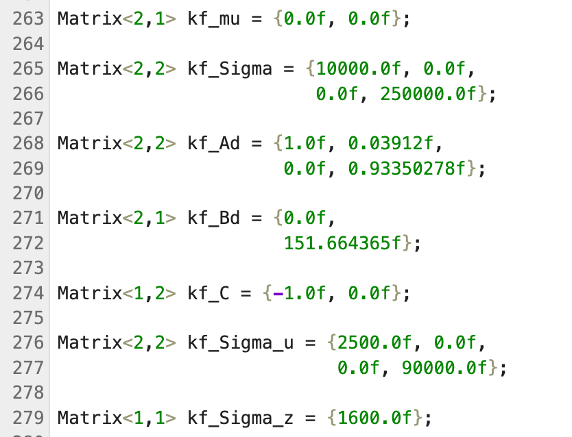
First, I added the BasicLinearAlgebra library to the Arduino side and defined the state, covariance, and system matrices required for the Kalman filter as global variables.
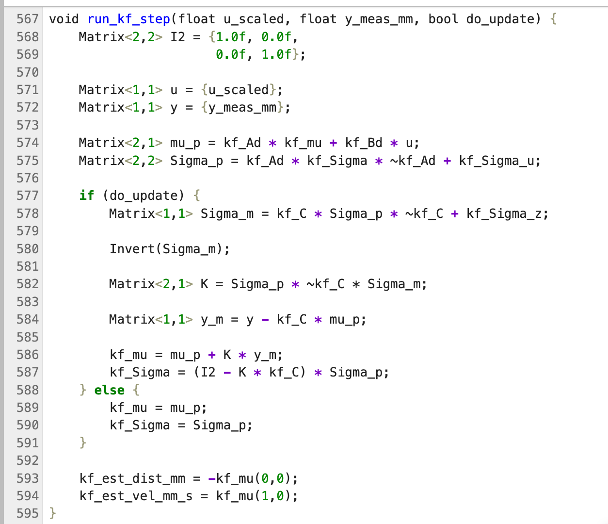
Subsequently, I implemented the same Kalman Filter prediction-update logic on the board as on the Python side.
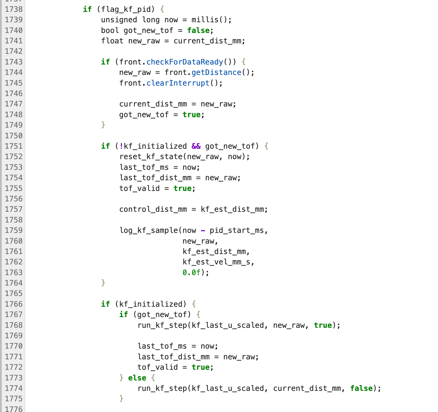
In the main loop, I have implemented the flag_kf_pid mode. In this mode, the first frame of ToF data is used to initialize the filter; subsequently, if new measurements are available, a Kalman filter update is performed, and if no new measurements are available, only a prediction is made. Therefore, the distance signal actually used by the PID is no longer the result of linear extrapolation, but rather kf_est_dist_mm.
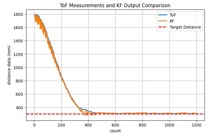
As can be seen in the figure, the KF output generally tracks the ToF curve well and remains stable as it approaches the target distance.
In addition, I recorded a video of the robot operating under KF-PID control.
Reference
I referenced Katherine Hsu's website.
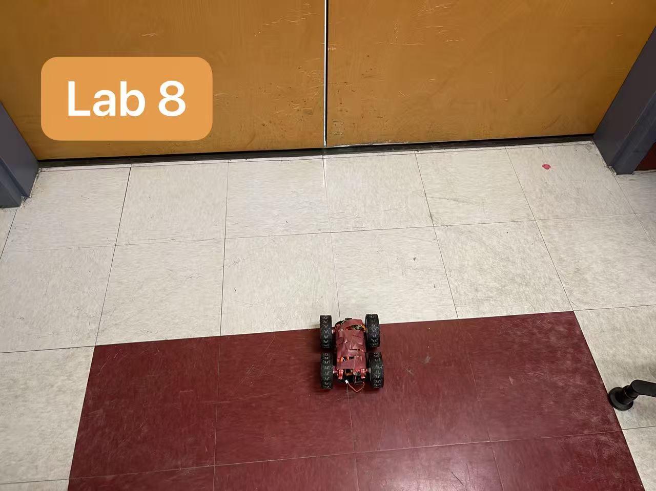
Lab 8: Stunts! (Drift)
For Lab 8, our goal was to perform the Drift stunt: the robot starts several meters away from the wall, drives forward at high speed, and initiates a 180 degree turn when it is within the target distance of the wall.
Task B: Drift
We reused the BLE command structure, the front ToF distance trigger, and the IMU/DMP yaw estimate from Lab 6. As a baseline for turn behavior, we used the orientation-control framework from Lab 6 and previously tuned yaw PID gains of approximately Kp = 0.8, Ki = 0.001, and Kd = 0.5.
I used a staged drift strategy:
Drive forward at a fixed fast PWM.
Use the front ToF sensor to detect when the robot is within the tuned trigger distance from the wall.
Initiate a fast turn using differential drive.
Track cumulative yaw using the IMU/DMP estimate.
Release the turn before the full 180 degree angle so that the robot’s remaining momentum carries it through the maneuver.
After fine-tuning the settings, I recorded three consecutive videos of drifting stunts.
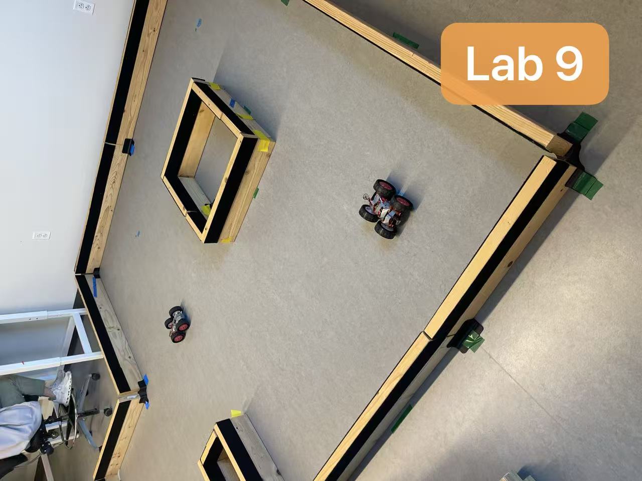
Lab 9: Mapping
Objective
The goal of this lab was to build a map of the front room of the lab using onboard ToF measurements collected while the robot rotated in place. I selected Option 2: PID control on orientation.
Orientation-Control Scanning
I implemented a step-scan controller on the Artemis. At the beginning of each scan, the robot stores the current DMP yaw as the starting heading. It then increments the target orientation by a fixed step size and reuses the Lab 6 orientation PID loop to rotate to the next angle. Once the yaw error is within tolerance, the robot stops, waits for a short settling interval, samples the front ToF sensor, logs the measured yaw and distance, and then proceeds to the next target angle. For my final scans, I used 20 degree increments and collected 18 readings per revolution.
Once the scan is active, the controller computes the wrapped yaw error to the next step target and uses the orientation PID loop to rotate on axis until the heading is within a small tolerance:
Because the DMP yaw wraps at \( \pm 180^\circ \), we also normalize angular quantities before using them in the controller:
float wrap_angle_deg(float ang) {
    while (ang > 180.0f) ang -= 360.0f;
    while (ang < -180.0f) ang += 360.0f;
    return ang;
}
Control Validation
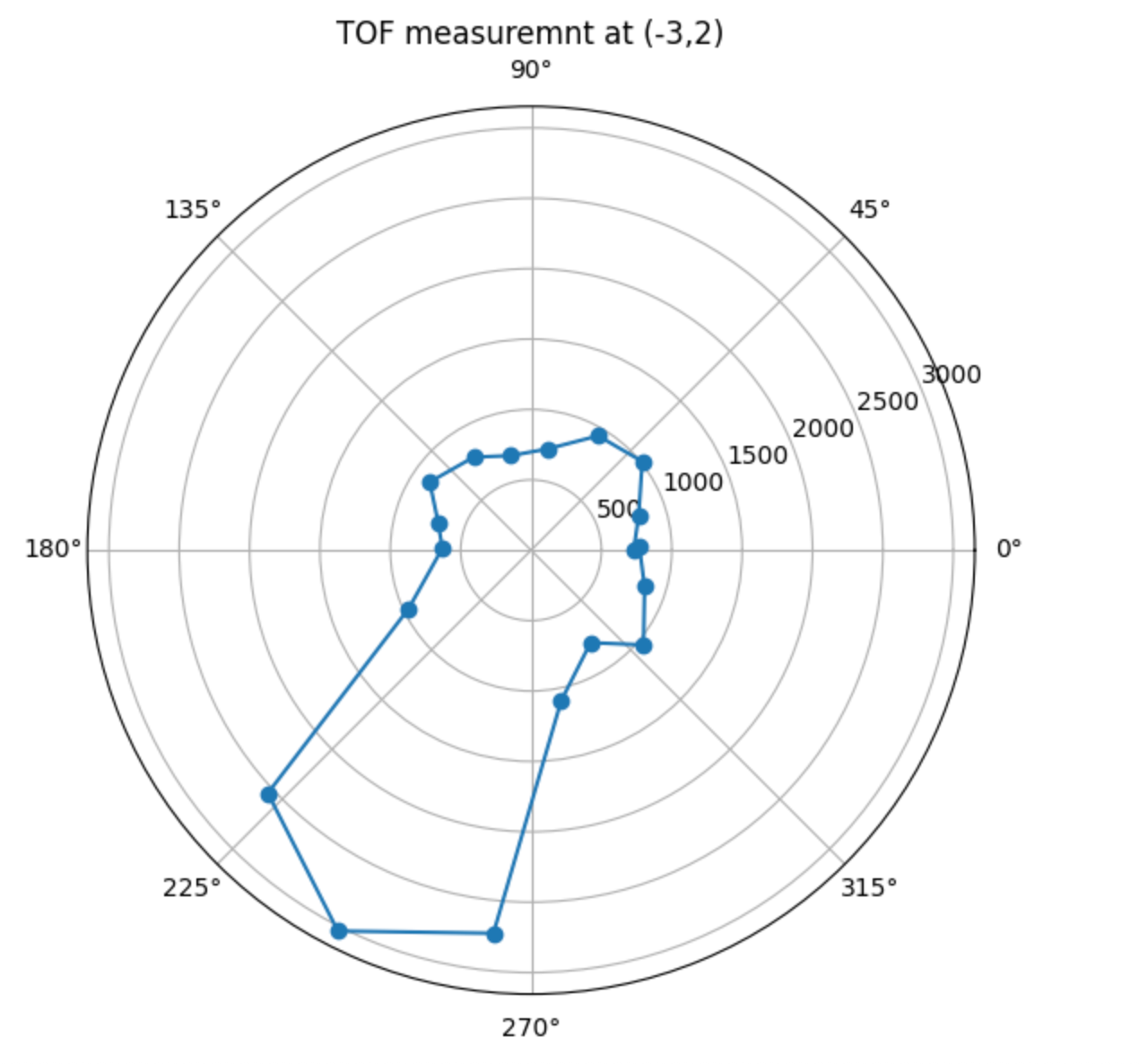
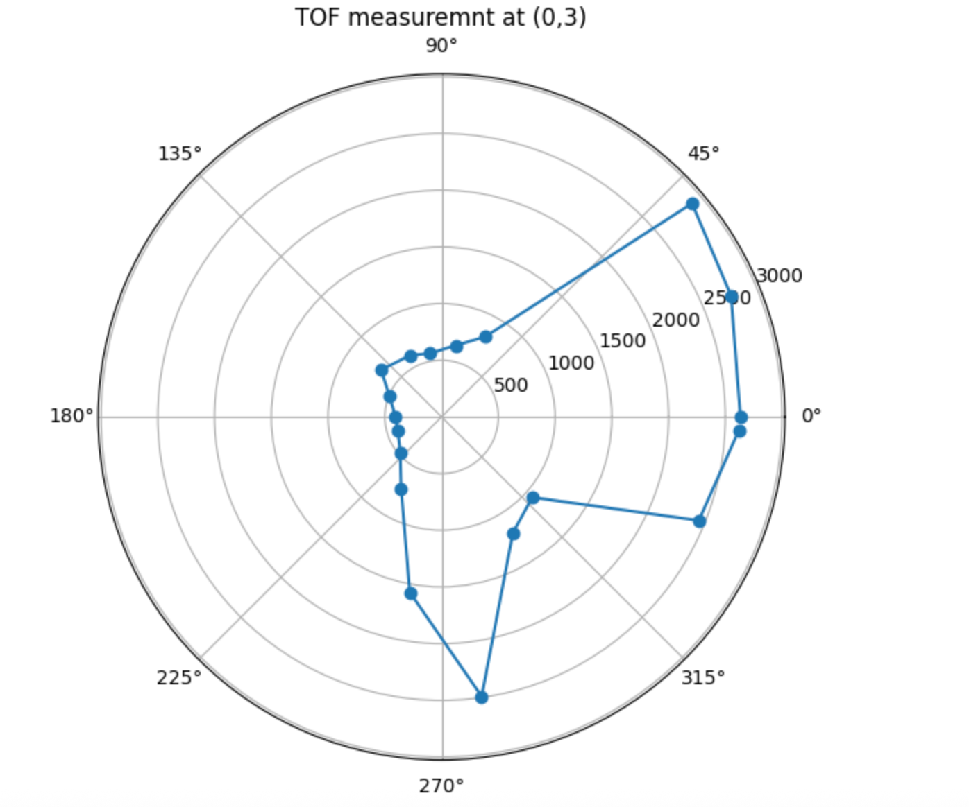
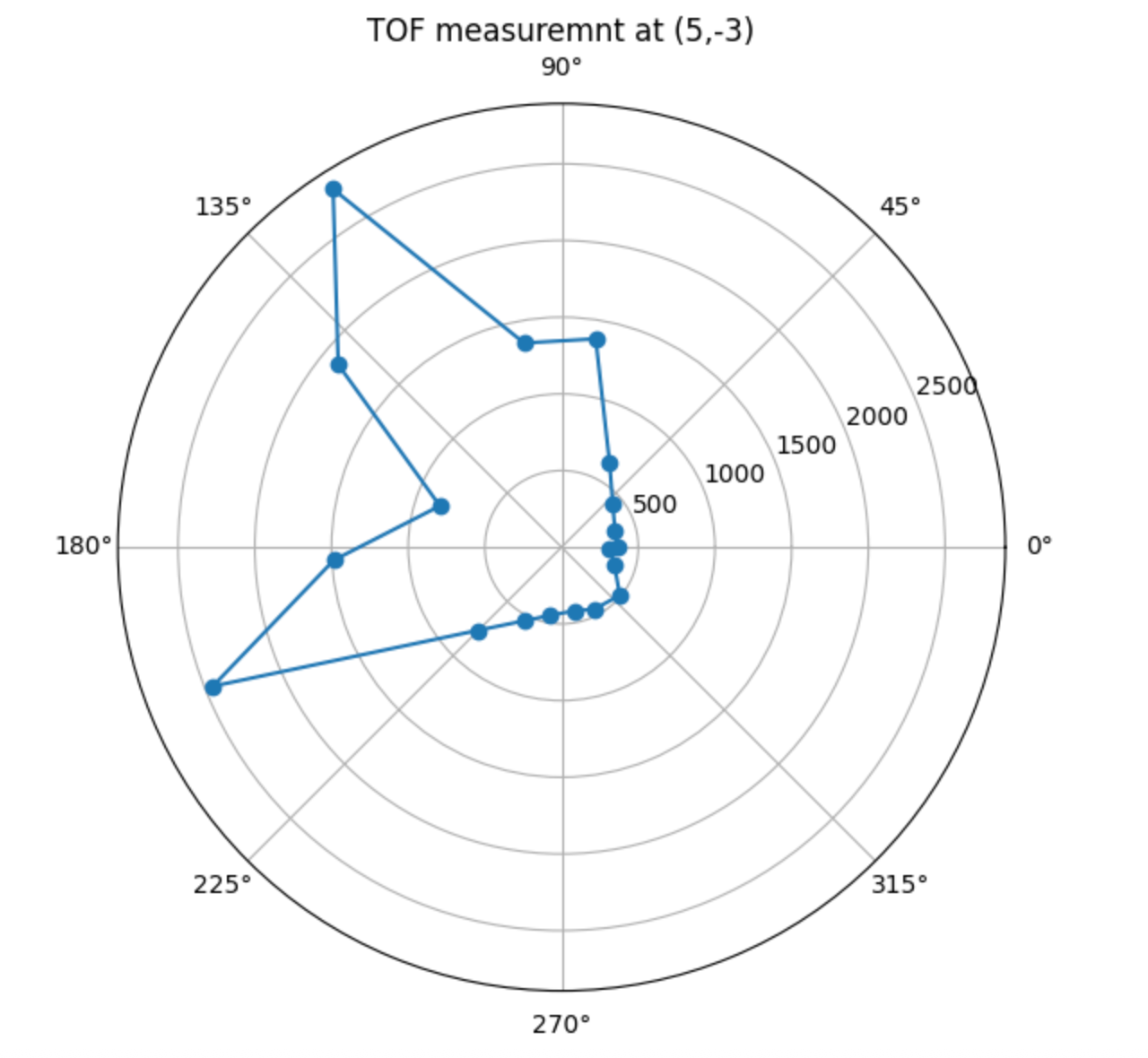
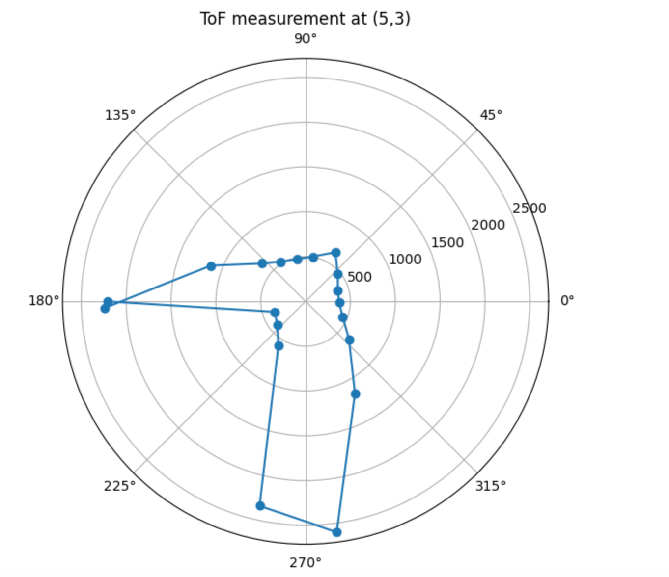
The robot was placed at each marked position in the lab: (-3,-2), (5,3), (0,3), and (5,-3). For every run, the robot began from a consistent physical starting orientation, rotated in place, and streamed the data back over BLE after completing the scan.
The single-position polar plots below were used as the required sanity checks.
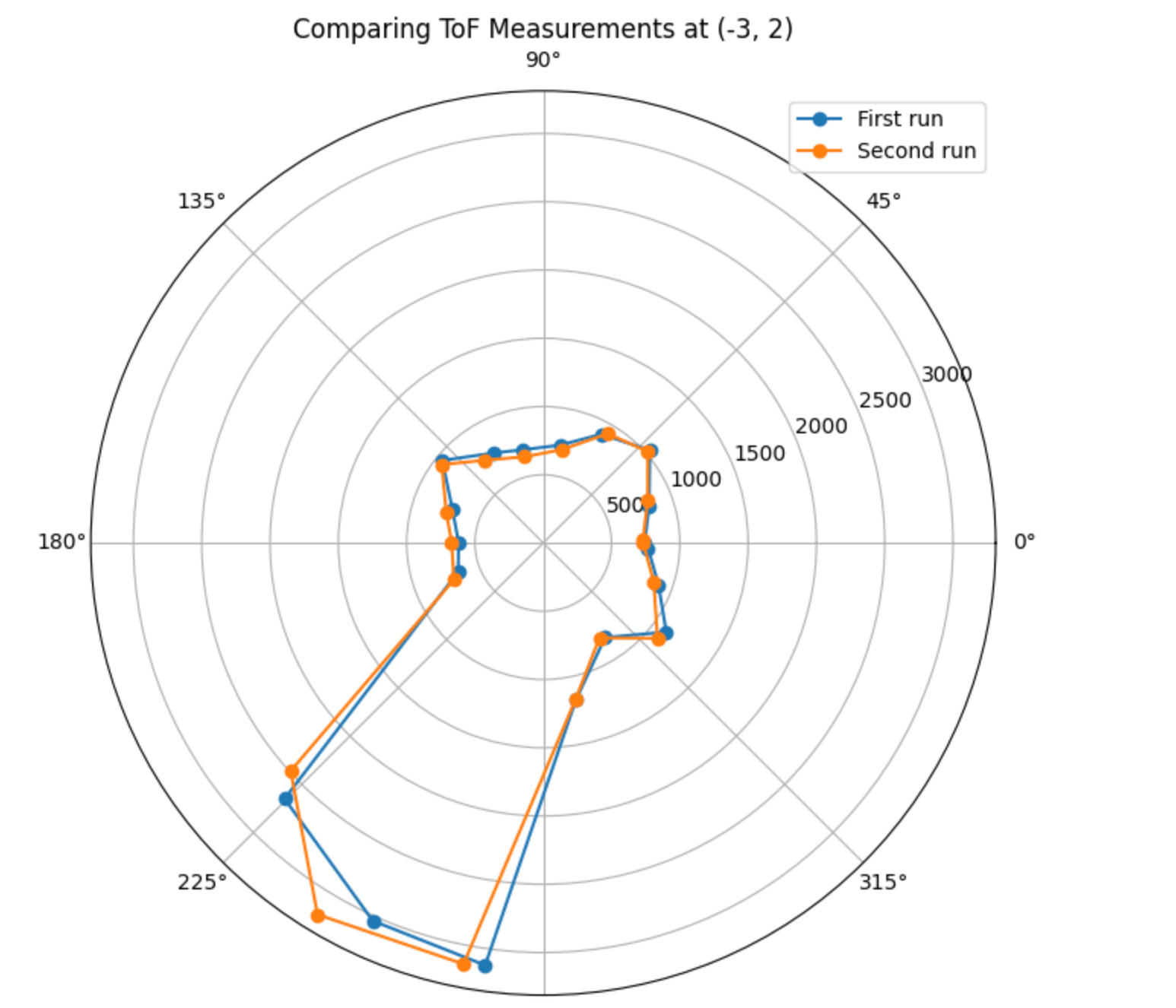
To check repeatability, I also repeated the scan at one location and overlaid the two polar plots. The two runs aligned closely, indicating that the orientation-controller-based stepping was consistent enough for mapping.
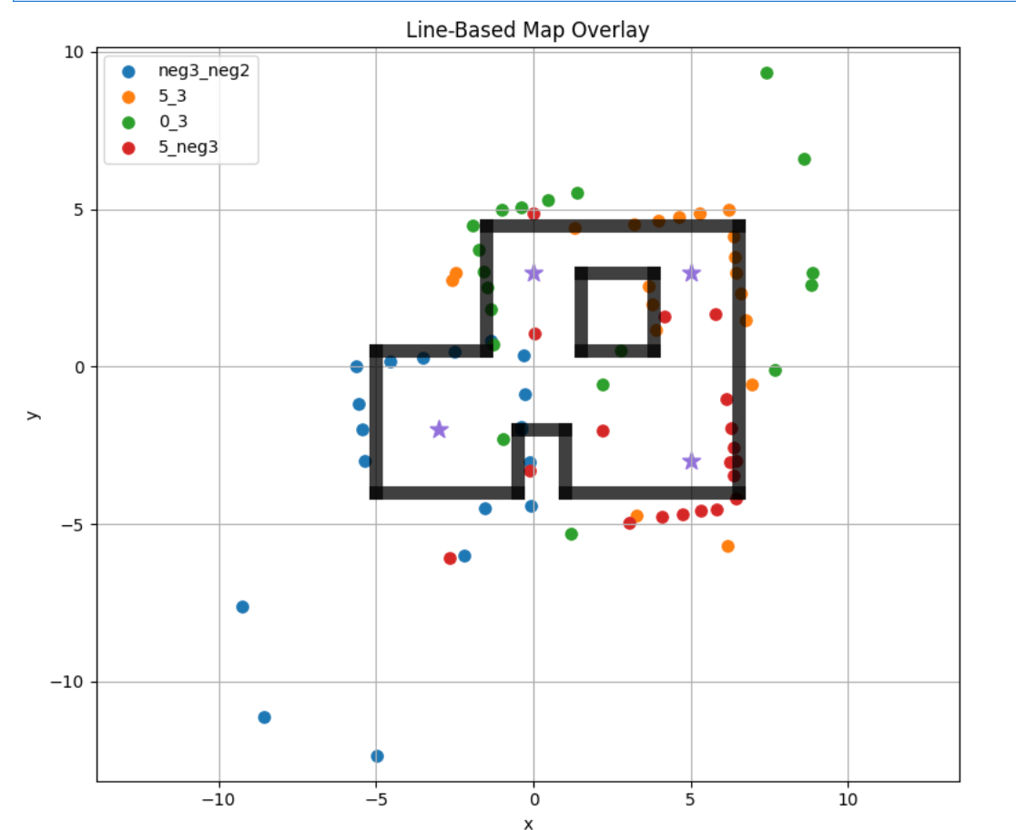
Transformation Matrices and World-Frame Conversion
After downloading the logs, I converted every ToF reading from the sensor frame into the room frame using homogeneous transforms. The front ToF sensor was mounted approximately 70 mm in front of the robot center, so I modeled that offset explicitly in the sensor-to-robot transform.
For each sample, I computed the robot-relative yaw from the logged DMP heading and then applied the sensor-frame transform followed by the robot-to-world transform:
After converting all four scans into the inertial frame, I plotted all points together with different colors.
Lab 10: Grid Localization Using Bayes Filter
Objective
The goal of this lab was to localize a virtual robot in a known map using a Bayes Filter. Instead of estimating pose in a continuous space, we discretized the state space into a 3D grid over \( (x, y, \theta) \). In this simulator, the grid size is \( 12 \times 9 \times 18 \), and the angle range is \( [-180, 180) \) degrees. At each step, the robot uses noisy odometry and 18 range observations collected during a full observation loop to estimate its most likely state.
Bayes Filter Algorithm
The Bayes Filter updates belief in two stages. First, the prediction step propagates the previous belief using the motion model:
Angle normalization was important here, since all headings must stay in \( [-180, 180) \).
def compute_control(cur_pose, prev_pose):
    """ Given the current and previous odometry poses, this function extracts
    the control information based on the odometry motion model.

    Args:
        cur_pose  ([Pose]): Current Pose
        prev_pose ([Pose]): Previous Pose

    Returns:
        [delta_rot_1]: Rotation 1  (degrees)
        [delta_trans]: Translation (meters)
        [delta_rot_2]: Rotation 2  (degrees)
    """
    x, y, yaw = cur_pose
    prev_x, prev_y, prev_yaw = prev_pose

    dx = x - prev_x
    dy = y - prev_y
    dyaw = yaw - prev_yaw
    delta_trans = np.hypot(dx, dy)

    if delta_trans < 1e-9:
        delta_rot_1 = 0.0
    else:
        delta_rot_1 = np.degrees(np.arctan2(dy, dx)) - prev_yaw

    delta_rot_1 = mapper.normalize_angle(delta_rot_1)
    delta_rot_2 = mapper.normalize_angle(dyaw - delta_rot_1)

    return float(delta_rot_1), float(delta_trans), float(delta_rot_2)
Odometry Motion Model
For the motion model, I compared the control implied by a candidate state transition with the actual odometry control. Each error term was evaluated with a Gaussian likelihood. This gives \( p(x_t \mid u_t, x_{t-1}) \).
def odom_motion_model(cur_pose, prev_pose, u):
    """ Odometry Motion Model

    Args:
        cur_pose  ([Pose]): Current Pose
        prev_pose ([Pose]): Previous Pose
        (rot1, trans, rot2) (float, float, float): A tuple with control data in the format
                                                   format (rot1, trans, rot2) with units (degrees, meters, degrees)


    Returns:
        prob [float]: Probability p(x'|x, u)
    """
    u_delta_rot_1, u_delta_trans, u_delta_rot_2 = u
    delta_rot_1, delta_trans, delta_rot_2 = compute_control(cur_pose, prev_pose)

    rot1_err = mapper.normalize_angle(delta_rot_1 - u_delta_rot_1)
    trans_err = delta_trans - u_delta_trans
    rot2_err = mapper.normalize_angle(delta_rot_2 - u_delta_rot_2)

    prob = (
        loc.gaussian(rot1_err, 0.0, loc.odom_rot_sigma)
        * loc.gaussian(trans_err, 0.0, loc.odom_trans_sigma)
        * loc.gaussian(rot2_err, 0.0, loc.odom_rot_sigma)
    )

    return float(prob)
Prediction Step of the Bayes Filter
In the prediction step, I looped over the discrete grid and accumulated transition probabilities into bel_bar. To reduce computation time, I skipped states whose prior belief was smaller than 0.0001. I also normalized bel_bar after the loop.
def prediction_step(cur_odom, prev_odom):
    """ Prediction step of the Bayes Filter.
    Update the probabilities in loc.bel_bar based on loc.bel from the previous time step and the odometry motion model.

    Args:
        cur_odom  ([Pose]): Current Pose
        prev_odom ([Pose]): Previous Pose
    """
    u = compute_control(cur_odom, prev_odom)

    x_cells = mapper.MAX_CELLS_X
    y_cells = mapper.MAX_CELLS_Y
    a_cells = mapper.MAX_CELLS_A

    loc.bel_bar = np.zeros_like(loc.bel, dtype=float)

    for prev_x in range(x_cells):
        for prev_y in range(y_cells):
            for prev_a in range(a_cells):
                prev_prob = loc.bel[prev_x, prev_y, prev_a]
                if prev_prob < 0.0001:
                    continue

                prev_pose = mapper.from_map(prev_x, prev_y, prev_a)

                for cur_x in range(x_cells):
                    for cur_y in range(y_cells):
                        for cur_a in range(a_cells):
                            current_pose = mapper.from_map(cur_x, cur_y, cur_a)
                            transition_prob = odom_motion_model(current_pose, prev_pose, u)
                            loc.bel_bar[cur_x, cur_y, cur_a] += prev_prob * transition_prob

    bel_bar_sum = np.sum(loc.bel_bar)
    if bel_bar_sum > 0.0:
        loc.bel_bar /= bel_bar_sum
Sensor Model \( P(z \mid x) \)
The sensor model used Gaussian likelihoods for the 18 range observations collected during the observation loop. For each grid state, I compared the expected observations with the measured data and computed the likelihood of each beam.
def sensor_model(obs):
    """ This is the equivalent of p(z|x).


    Args:
        obs ([ndarray]): A 1D array of expected sensor observations for a specific pose in the map

    Returns:
        [ndarray]: Returns a 1D array of size 18 (=loc.OBS_PER_CELL) with the likelihoods of each individual sensor measurement
    """
    range_data = np.squeeze(loc.obs_range_data)
    prob_array = np.zeros(mapper.OBS_PER_CELL)

    for i in range(mapper.OBS_PER_CELL):
        prob_array[i] = loc.gaussian(obs[i], range_data[i], loc.sensor_sigma)

    return prob_array
Update Step of the Bayes Filter
The update step multiplies the prior bel_bar by the sensor likelihood and then normalizes the result. Normalization was necessary for both bel and bel_bar, otherwise the values would not remain a valid probability distribution.
def update_step():
    """ Update step of the Bayes Filter.
    Update the probabilities in loc.bel based on loc.bel_bar and the sensor model.
    """
    x_cells = mapper.MAX_CELLS_X
    y_cells = mapper.MAX_CELLS_Y
    a_cells = mapper.MAX_CELLS_A

    loc.bel = np.zeros_like(loc.bel_bar, dtype=float)

    for x in range(x_cells):
        for y in range(y_cells):
            for a in range(a_cells):
                obs = mapper.get_views(x, y, a)
                prob_array = sensor_model(obs)
                loc.bel[x, y, a] = np.prod(prob_array) * loc.bel_bar[x, y, a]

    bel_sum = np.sum(loc.bel)
    if bel_sum > 0.0:
        loc.bel /= bel_sum
    else:
        loc.bel = np.copy(loc.bel_bar)
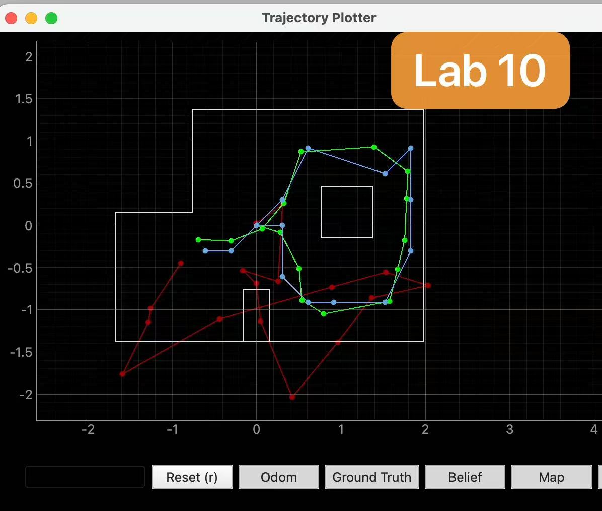
Comparison / Results
Without Bayes Filter, odometry drift is clearly visible. The estimated trajectory gradually deviates from the robot’s true position, and the motion becomes less reliable over time because the error keeps accumulating.
With Bayes Filter, the belief trajectory is much closer to ground truth, and localization is more stable. The most probable state after each iteration gives a reasonable estimate of the robot pose, especially when the robot is near walls or other distinctive parts of the map where the range observations are more informative.
The method still has limitations. If observations are not distinctive enough, if the grid resolution is coarse, or if odometry error becomes too large, the estimated pose can still drift or converge to a nearby but incorrect state. Overall, the filter works best when motion and observation information complement each other.
Lab 11: Localization on the Real Robot
Objective
The goal of this lab is to run Bayes-filter localization on the real robot and compare the real-robot results with the simulator.
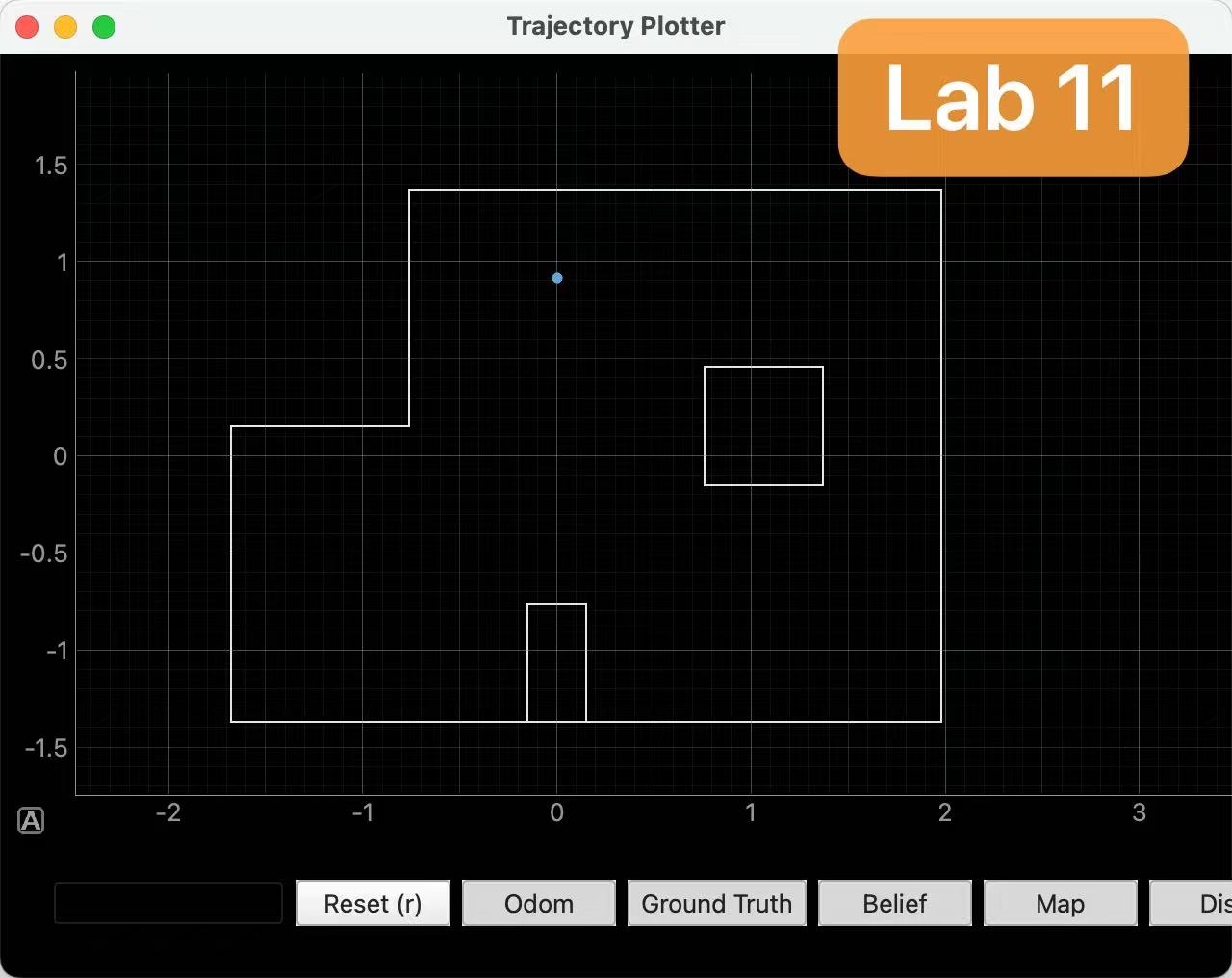
Grid Localization
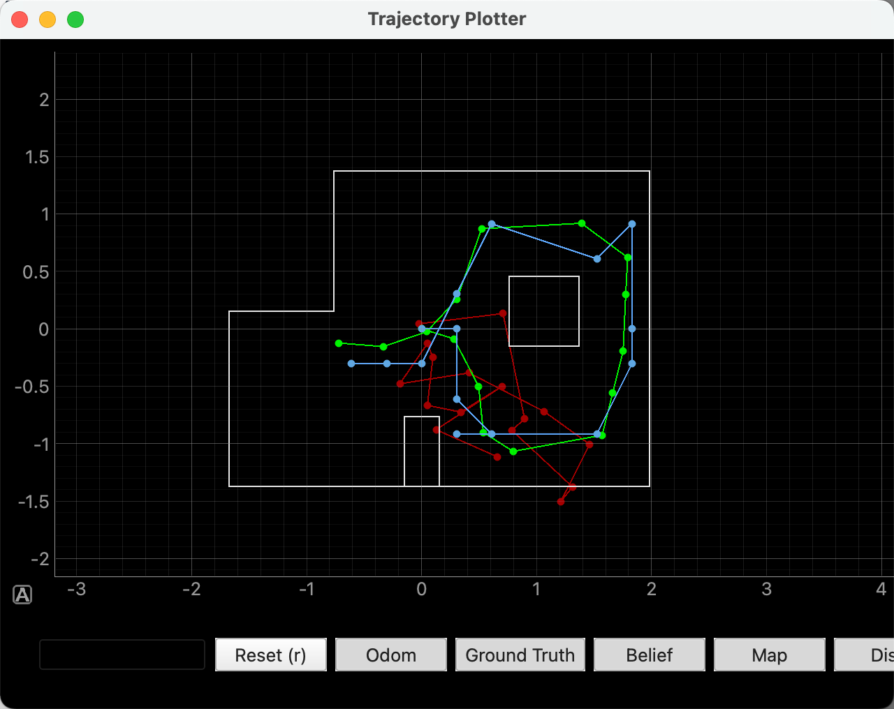
The plot below shows the simulation result from lab11_sim.ipynb. The blue trajectory represents the belief, the red trajectory represents odometry, and the green trajectory represents ground truth. As in the simulator, the belief remains much closer to the ground-truth path than raw odometry alone, which provides a useful baseline before moving to the real robot.
Jupyter Notebook Implementation
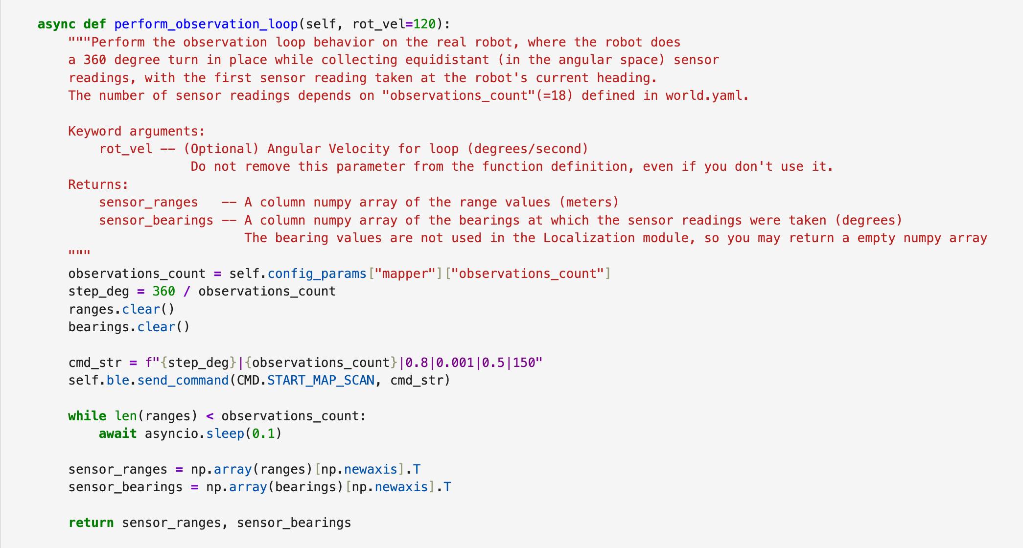
For the notebook side, I implemented RealRobot.perform_observation_loop(). This function commands the robot to perform a full in-place scan while collecting ToF measurements every 20 degrees, and then returns the readings as NumPy column arrays for the localization module.
The function sends START_MAP_SCAN to the robot and waits until all 18 readings have been received. The command string sets the step size, number of observations, and the PID gains used during the observation loop.
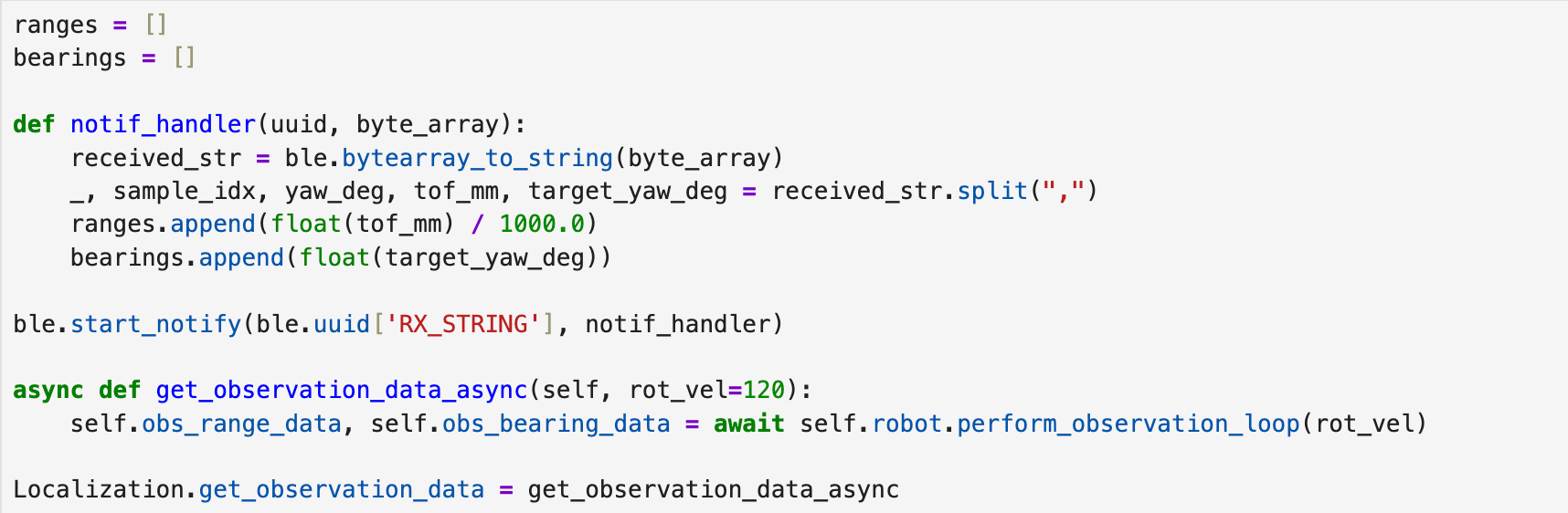
I also added a BLE notification handler to receive the data streamed back from the robot. Since the observation data is collected through asynchronous BLE callbacks, I converted get_observation_data() into an async function and called it with await in the notebook.
For each marked pose, I reset the plotter, initialized a uniform belief, executed one full observation loop, ran a single update step, and then manually plotted the measured ground-truth position. Since the marked poses in the lab are specified in feet while the plotter expects meters, I converted each coordinate by dividing by 3.281.
Robot-Side Scan Direction
The handout requires the observation loop to move in the counter-clockwise direction, with the first measurement taken at the robot’s current heading. My Lab 9 scan code originally incremented the setpoints in the opposite direction, so for Lab 11 I changed the firmware setpoint generation to step through decreasing yaw targets. I kept the rest of the scan state machine unchanged.
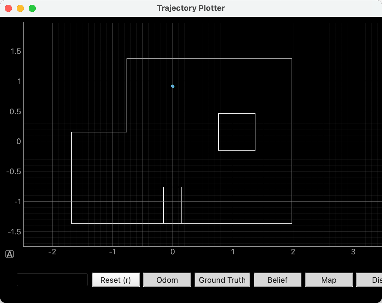
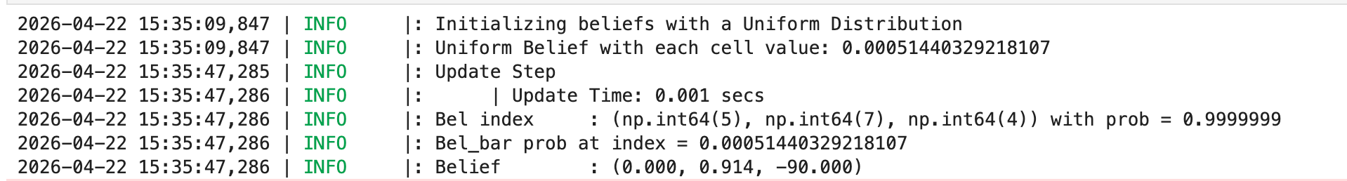
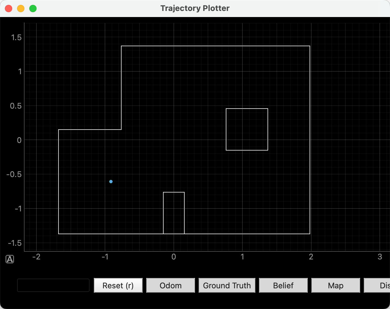
This was one of the cleanest trials. The belief returned by the update step was (0.000, 0.914, -90), which matches the ground-truth position exactly in x and y. In the plot, the blue and green points lie on top of each other, so only one point is visually obvious. This suggests that the observation loop produced a very distinctive signature at this pose.
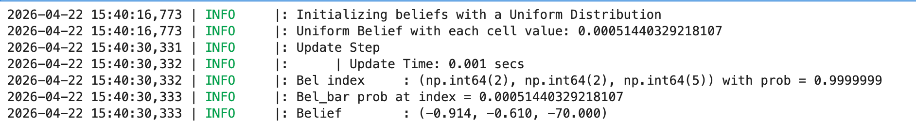
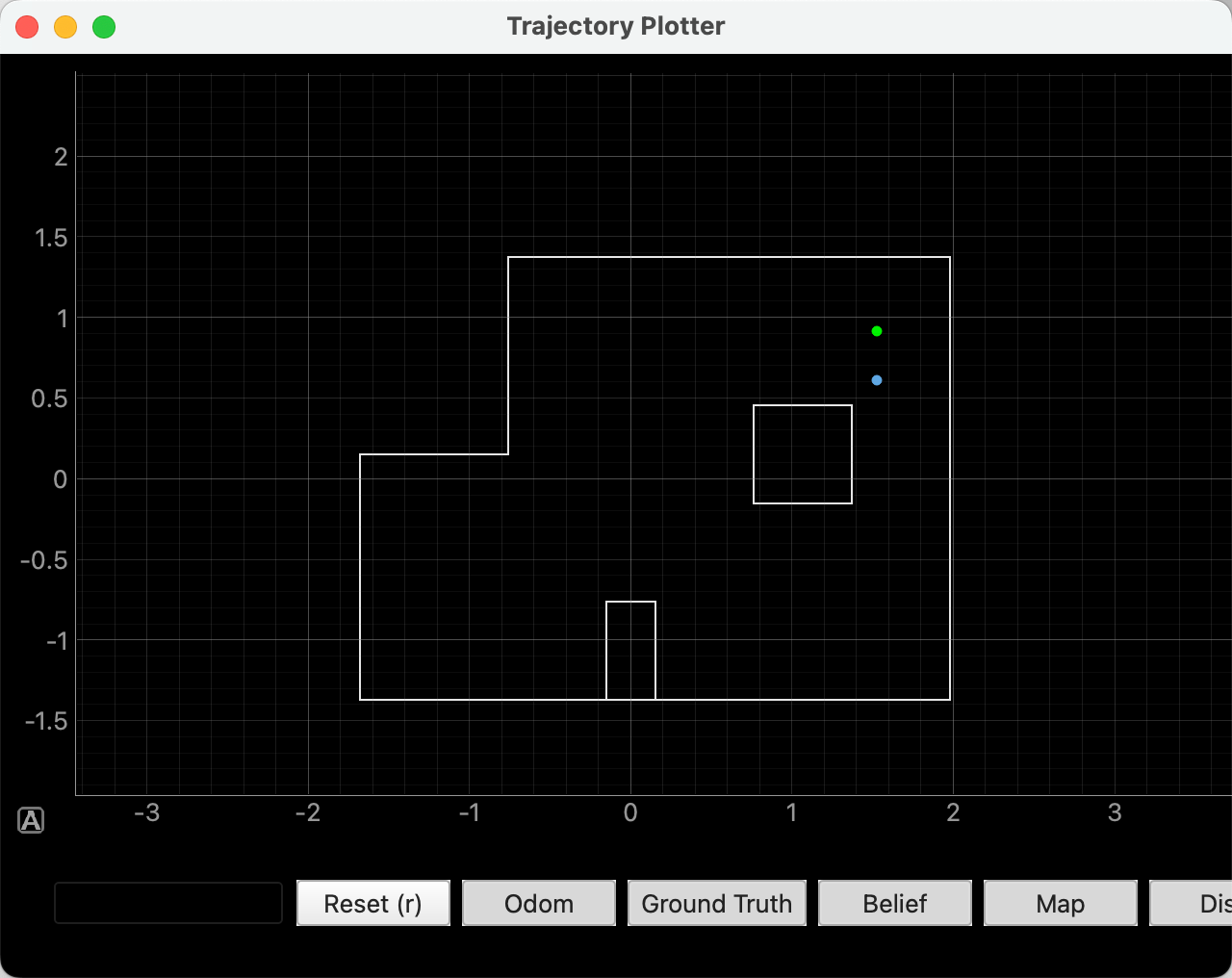
(-3, -2)
This marked pose also localized very well. The belief was (-0.914, -0.610, -70), so the position matched the measured ground truth exactly even though the heading estimate was offset. The overlap between the belief and the ground truth again makes the plot appear as if it contains only one point. Among the four positions, this pose and (0,3) were the most reliable in translational accuracy.
(5, 3)
At (5, 3), the x coordinate localized correctly, but the y coordinate was biased downward by about 0.30 m. The result is still in the correct region of the map and close to the correct wall, but it is not as precise as the two left-side trials. This suggests that the right side of the map is somewhat less distinctive under a single update-only scan.
(5, -3)
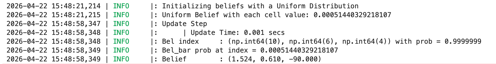
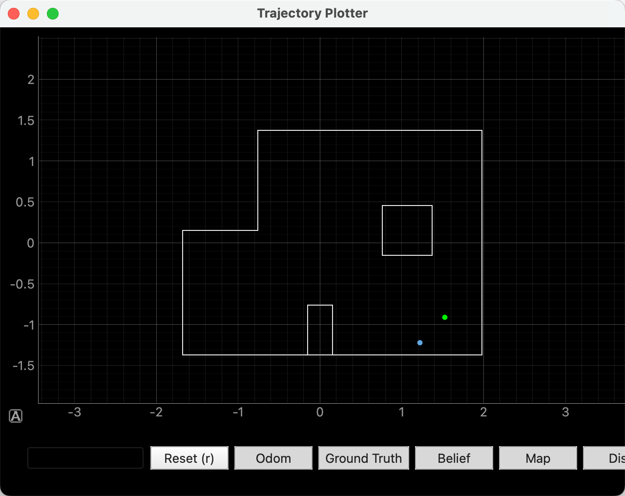
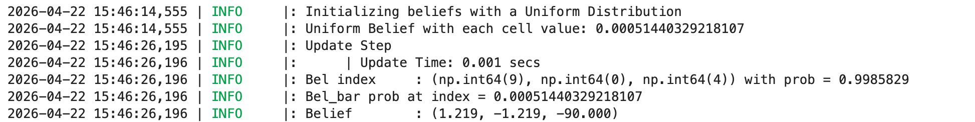
This was the weakest of the four marked poses. The localized belief (1.219, -1.219, -90) still landed in the bottom-right portion of the map, but it shifted diagonally inward from the measured ground truth by about 0.43 m. Since Lab 11 uses only a single update step on real data, this kind of ambiguity is not surprising when two regions of the map have somewhat similar range structure.
References
I referenced Katherine Hsu’s Fast Robots website while organizing this write-up.
Lab 12: Path Planning and Execution
Objective
The goal of Lab 12 was to make the robot navigate through the course waypoints as quickly and accurately as possible. I used the given map and waypoint sequence, but instead of running a full replanning/localization loop during the final demo, I implemented a preset waypoint executor that was more reliable for my hardware.
The lab was intentionally open-ended, so I considered two directions. The first was a full local-planning pipeline that would repeatedly scan, localize, and replan. This was attractive because it would reduce accumulated error, but each scan took a long time and introduced more failure modes during the live run. The second direction was a simpler turn-and-drive strategy using the known waypoint list. I chose the second approach for the final demonstration because the map and waypoints were fixed, and the robot became much more repeatable after tuning the turn controller and drive timing.
Waypoint Path
The robot followed the required path in feet: (-4,-3), (-2,-1), (1,-1), (2,-3), (5,-3), (5,-2), (5,3), (0,3), and (0,0). The map below uses the wall geometry from world.yaml and overlays the preset route.
The first segment starts diagonally, so I manually placed the robot at (-4,-3) with an initial heading of about 45 degrees. After that, every segment is represented as a relative turn followed by a straight drive. This matched the turn-go-turn procedure from the odometry model, but I skipped the final turn at each waypoint because the next segment's heading computation already handles the required orientation change.
The laptop handled the high-level path computation in Jupyter. For each pair of waypoints, Python computed the segment heading, relative turn angle, distance, and drive time. The Arduino only executed motion primitives sent over BLE. This kept the onboard code simple and made tuning faster.
This split was useful during testing. When a segment overshot or a turn was too aggressive, I could change the notebook parameters and rerun only one segment without reflashing the robot. The Arduino firmware only needed to support reliable primitive commands, while the notebook handled path sequencing, logging, and emergency stop commands.
I added four Lab 12 BLE commands: TURN_REL_DEG, DRIVE_CELL_MM, STOP_NAV, and SEND_NAV_LOG. Turning is closed-loop using the DMP yaw estimate. Straight driving is mostly open-loop: the distance is converted to a calibrated motor runtime using ms_per_ft. ToF is used as a safety stop, not as the primary distance controller.
The turn command is relative rather than absolute. For example, a command of 45 degrees means “turn 45 degrees from the current DMP yaw,” not “turn to global yaw 45.” The robot reports TURN_STARTED with the start yaw and target yaw, then reports TURN_DONE when the yaw error is small and stable. For driving, the firmware records the starting yaw and can apply a small heading correction, but in the final route I relied mainly on low speed and timed motion for distance repeatability.
The largest tuning issue was overshoot during turns. The robot could enter the yaw tolerance and still coast farther after the motors stopped. To fix this, I lowered the turn PWM range to 100-130 and required the yaw error to stay within 3 degrees for 180 ms. For straight driving, I empirically tuned base_pwm=46 and ms_per_ft=750. This reduced accumulated distance error enough to complete the full route.
I also reduced the amount of data requested during the full run. Earlier versions fetched the full navigation log after every turn and drive, which added a noticeable delay between segments. For the final run, collect_nav_log was disabled by default, so the robot only waited for the compact status messages such as TURN_DONE and DRIVE_DONE. This made the path execution smoother while still writing a JSONL summary for the report.
Final Run Parameters
Parameter
Value
Purpose
base_pwm
46
Slow straight driving with enough torque
ms_per_ft
750
Open-loop distance calibration
front_stop_mm
10
Emergency stop threshold kept low for final route
turn_kp, turn_ki, turn_kd
0.8, 0, 0.5
DMP yaw PID tuning
turn_timeout_ms
8000
Allows slower stable turns
Execution Summary
In the best logged run, all eight motion segments completed with DRIVE_DONE. The longest straight sections were the 5 ft runs from (5,-2) to (5,3) and from (5,3) to (0,3), each using 3750 ms of drive time.
The log confirms that the mission reached the final waypoint sequence without triggering a ToF stop or turn timeout in the successful run. The total route is still sensitive to placement error at the start, because every straight segment is timed. However, using slower motion reduced sliding after stops and made the later waypoints more consistent than the faster early trials.
Segment
Distance
Drive Time
Status
1: (-4,-3) to (-2,-1)
2.828 ft
2121 ms
Done
2: (-2,-1) to (1,-1)
3.000 ft
2250 ms
Done
3: (1,-1) to (2,-3)
2.236 ft
1677 ms
Done
4: (2,-3) to (5,-3)
3.000 ft
2250 ms
Done
5: (5,-3) to (5,-2)
1.000 ft
750 ms
Done
6: (5,-2) to (5,3)
5.000 ft
3750 ms
Done
7: (5,3) to (0,3)
5.000 ft
3750 ms
Done
8: (0,3) to (0,0)
3.000 ft
2250 ms
Done
Run Videos and Analysis
Run 1 shows the early behavior of the preset path. The robot follows the route structure, but small straight-line distance errors begin to accumulate because the drive distance is still open-loop.
Run 2 shows another complete attempt with the same streamlined command flow. The robot pauses only briefly between segments because the full navigation log is not requested during normal execution, and the tuned turn controller keeps the heading changes controlled.
Run 3 is another representative run of the same implementation. Like the other trials, it uses the Jupyter-generated segment commands, the relative-yaw turn primitive, and the calibrated time model for straight driving.
Run 4 is the final demonstration run. The robot reaches the waypoint sequence using closed-loop turns and calibrated open-loop drives. This is the run that best represents the final implementation: simple offboard planning, reliable onboard yaw control, and conservative straight-line speed.
Limitations
The main limitation is that straight-line distance is not closed-loop. Without wheel encoders, the robot cannot directly measure how far it traveled, so battery level and floor friction can still change the result. However, the combination of reliable yaw turns, conservative speed, and calibrated drive timing was sufficient for a complete Lab 12 run.
A more advanced version would add correction after selected waypoints. One option would be to use ToF measurements as a local landmark when the robot faces a known wall, or to run a Lab 11 localization scan after major turns. I did not use this in the final run because the extra scan time made the demonstration less robust, but it would be the natural next step for reducing accumulated open-loop drift.